Munich Personal RePEc Archive
Waiting to Cooperate?
Kaplan, Todd and Ruffle, Bradley and Shtudiner, Zeev
Universities of Exeter and Haifa, Wilfrid-Laurier University and
Ben-Gurion University, Ariel University
22 September 2013
Online at
https://mpra.ub.uni-muenchen.de/50096/
Waiting to Cooperate?
Todd R. Kaplan
University of Exeter University of Haifa
Bradley J. Ruffle
Wilfrid Laurier University Ben-Gurion University
Ze'ev Shtudiner
Ariel University
September 2013
Abstract
Sometimes cooperation between two parties requires exactly one to cede to the other. If the decisions whether to cede are made simultaneously, then neither or both may acquiesce leading to an inefficient outcome. However, inefficiency may be avoided if a party can wait to see what the other does. We experimentally test whether adding a waiting option to such a two-player cooperation game enhances cooperation. Although subjects cede less overall with the waiting option, we show that they coordinate more and consequently achieve higher profits. Yet, a dark side overhangs waiting: the least cooperative pairs do worse with this option. They wait not to facilitate coordination but to disguise their entry.
1. Introduction
Cooperation often plays a central role in achieving social surplus. One type of
cooperation requires that one person cedes to another with the thought that the other
person will in turn cede in the future. Bidding behavior in procurement auctions,
competition for market share and entry decisions between firms with multimarket contact
all share this property. In these examples, if each group member has a private value that
derives from the situation (such as the item's value in an auction or the profitability of a
particular market) and the values of all players are observable, the maximum joint profit
When players’ values are private information, coordinating on efficient cooperation is
more difficult. For example, suppose two fast-food chains each contemplate opening a
franchise in a small town. They may possess different expected private values of being
the local monopolist that stem from different expected costs or demand for its products. If
these two chains wish to collude implicitly, then the chain with a low value would stay
out, under the presumption that the favor will be returned in the future.
With values to being a local monopolist private and direct communication between
the chains illegal, this form of cooperation cannot be realized. Instead, both chains may
decide to enter the market or both may stay out. The possibility of waiting enables the
chains to coordinate more efficiently. To illustrate, if a firm always enters for a certain
range of high values, then the possibility of waiting permits the firm to refine its strategy
to entering on only a subset of this range and waiting otherwise. By waiting and
subsequently not entering whenever the other enters, double entry is avoided and higher
social surplus attained.1
In this paper, we analyze experimentally how the inclusion of a waiting option
affects cooperative play. The starting point is Kaplan and Ruffle (2012). In their
two-player, repeated cooperation game, each player privately receives a randomly drawn
integer between 1 and 5 with equal probability in each round. Upon receipt of the integer,
each player must decide between one of two actions: enter or exit. By exiting a player
receives zero. By entering, he receives his number if his partner exits and one-third of his
number if his partner also enters.2 In this game, entry (non-cooperation) is the unique dominant strategy, but the social optimum is obtained when only the player with the
higher value enters (or just one enters in the case of a tie). We conduct this treatment for
60 rounds with fixed pairs.3 Both players’ values are made public after each round.
1
For example, suppose the set of values is 1, 2 and 3 with an equal chance of each. If firms enter on a 2 or 3, then double entry occurs 4/9 of the time, no entry 1/9 of the time and single entry the remaining 4/9. By switching to entry on 3 and waiting on 2, double entry occurs only 1/9 of the time initially (when both have 3s) and another 1/9 after waiting (when both have 2s). Single entry increases to 2/3 of the time with no entry still at 1/9.
2
While we refer to the other pair member as the "partner" for brevity, the experimental instructions invoke the more neutral phrase "the person with whom you are paired".
3
We conduct this game under two experimental treatments that differ in the number of
stages available to players when deciding whether or not to enter. In the Now treatment,
players must decide simultaneously in a single stage between enter and exit. Play in Now
is compared to play in a second two-stage game where players are given the option of
waiting. We refer to this treatment as “Wait.” In stage one of Wait, each player decides
between one of three actions: enter, exit or wait. By waiting, the player avoids
committing to entering or exiting in stage 1. Instead, he observes his partner’s stage-one
decision and then decides in stage two between one of two actions: enter or exit.
Based upon whether players ultimately enter or exit, the payoff structure in Wait is
identical to that in Now: by exiting in either stage, the player receives zero. By entering in
either stage, he receives his number if his partner exited in either stage 1 or stage 2 and
one-third of his number if his partner also entered in either stage. In Wait, entry remains
the unique dominant strategy, while the social optimum again consists of only the player
with the higher value entering. Note that if players choose not to make use of the waiting
option in the first stage, the game reduces to Now.
Overall, we find that although Wait leads to a higher percentage of entry (a sign of
reduced cooperation), it also attains a higher degree of efficient cooperation (where the
player with the higher number enters and the player with the lower number stays out) and
higher average profits than Now. The cooperation and profit improvements occur since
many subjects use the waiting option to coordinate more efficiently. For example, many
subjects who see their partner enter in stage 1 opt to exit in stage 2 to prevent double
entry.
While there are clear improvements for some subjects and the overall average
profits, the cumulative distributions of the pair profits for the two treatments intersect
near 50%. More specifically, the pair profits in the lower half of Now stochastically
dominate those of Wait. A closer look at the data points to malevolent uses of the waiting
option. Low-profit subjects who wait in the first stage often enter in the second stage
regardless of their value and their partner's first-stage decision, thereby illustrating the
potential for the cooperation-enhancing waiting option to backfire.
Our paper contributes to several strands of literature. The addition of the wait option
relates to the endogenous timing literature. In Cournot duopolies, when the timing of
quantity decisions is endogenous, players may postpone their decisions in order to make
strategic use of other players' actions (see, for example, Hamilton, and Slutsky 1990).
Likewise, when publicly observable decisions reveal agents' private information, strategic
delay of decisions may also be an equilibrium (see Chamley and Gale 1994; Gul and
Lundholm 1995). Attempts to observe strategy delay in the laboratory have met with
mixed results (Huck, Muller, and Normann 2001, 2002; Potters, Sefton and Vesterlund
2004; Ziegelmeyer et al. 2005; Fonseca and Normann 2008). In our environment, we find
that the waiting option is indeed exploited but not always to increase cooperation.
Our paper also contributes to the tragedy of the commons literature (see Dietz, Ostrom,
and Stern 2003) and the ability of institutions to facilitate cooperation (see Scholz and
Gray 1997; Ostrom 2009). First, our game is a stylized version of a discretized tragedy of
the commons dilemma: one can either fish or not fish, for instance. The social optimum
requires a reduction of fishing. While the cooperative solution to the tragedy of the
commons requires that both parties curtail fishing to avoid depletion of the resource, the
cooperative solution in our game entails exactly one party choosing not to fish. In repeated
settings, the implicit use of budgets to manage one’s actions can help achieve cooperation.4 Staying out in some periods when one has low values allows one to build goodwill that can
be beneficial in periods in which one has a high value and wishes to enter. This possibility
relates to work experimental work on the tragedy of the commons where self-governance
is possible (e.g., Ostrom, Walker and Gardner 1992).
The addition of the wait option to our game allows us to examine how an
institutional change can affect cooperation among parties. Our Wait treatment parallels
institutions in which others' actions are more transparent, while Now is more similar to
institutions in which the moves of others are opaque.
The next section introduces the experimental design, treatments and possible
strategies. In section 3, we detail the experimental procedure. We present the results in
section 4. Section 5 concludes.
4
2. Experimental Design
2.1. Treatments
The experiments were conducted in z-Tree (Fischbacher 2007) with fixed pairs for 60
rounds preceded by five practice rounds in different pairings. Each subject in the pair
privately receives an independently and randomly drawn integer between 1 and 5 in each
round. We conducted two treatments that differ in the number of stages. The control
treatment Now consists of a single stage in which players simultaneously decide whether
to enter or exit. The decision to exit yields 0, whereas entry yields the value of the
number if the partner exits and 1/3 of the value of the number if the partner also enters
(see Table 1 for a summary of the payoffs). After each round, subjects observe their
partner's decision and value. The second treatment, Wait, consists of two stages. In the
first stage, each player decides simultaneously whether to enter, exit or wait. Waiting in
stage 1 allows the subject to observe his partner's stage-one decision before deciding in
stage 2 whether to enter or exit. Waiting is costless; the payoffs depend only on the
players’ final decisions to enter or exit. Thus, the payoff structure is identical to that in
Now.
Wait affords more favorable conditions for cooperation. If the partner enters or exits
in stage 1, a cooperative subject who waits simply chooses the opposite action in stage 2.
If both wait, the game reverts to a one-stage game, but with potentially different beliefs
about each other’s values. For example, if a subject consistently waits only with a 3 or 4,
after seeing him wait, his partner would believe that the subject has an equal chance of
either value rather than an equal chance of a 1, 2, 3, 4 and 5 as in Now.
2.2. Environment and hypothesis
The theoretical framework and properties of the one-stage game are presented in Kaplan
and Ruffle (2012). There are non-cooperative and cooperative solutions to this game. The
Bayes-Nash equilibrium is to follow the dominant strategy of always entering for values
greater than zero (i.e., for all values in the present game). One cooperative solution is for
take the form of players taking turns entering and exiting.5 The pair's expected payoff from playing the alternating strategy is 3. Another cooperative solution is for both players
to enter only with high numbers, such as 3, 4 and 5. This cutoff strategy yields a slightly
lower expected payoff of 2.88. Notwithstanding, Kaplan and Ruffle (2012) find it to be
the modal strategy.
In Wait, a stage-one strategy maps values into the possible actions of enter, exit or
wait. Full cooperation (maximizing a pair's joint profits) entails monotonic stage-one
strategies. Namely, if the action for value x is enter, then the action for all values v>x is
also enter. Also, if the action for value x is wait, then the action for all values v>x is
either wait or enter (see Appendix A for the proof). It is worth noting that, in contrast to
Now in which alternating is the joint-payoff-maximizing strategy, turn taking between in
stage 1 can never be part of the social optimal in Wait (see the last paragraph of
Appendix A for the proof).
Table 2 displays the joint expected payoffs for all possible pairings of the 21
monotonic strategies and alternating. To describe the monotonic strategies, we use the
following notation: the player exits with values to the left of the parentheses, waits with
values between the parentheses, and enters with values to the right of the parentheses. For
example, a player who employs the strategy 12(34)5 exits when he receives a value of 1
or 2, waits when he receives a value of 3 or 4, and enters when he receives a value of 5. If
a player waits in the first stage, he enters in the second stage if the other player exited in
the first stage and exits if the other player entered in the first stage. If both players chose
to wait in the first stage, it is assumed that they employ the alternating strategy to resolve
which one enters in stage two.6
Table 2 shows that several pairs of strategies achieve the highest joint expected profit
of 3.60: 123()45-(12345), 12(3)45-(12345), 12()345-(12345), where the dash separates
player 1’s strategy from player 2’s. This profit compares favorably with the
full-information first-best expected surplus (i.e., only the player with the higher value enters)
5
Turn taking has been observed in Zillante (2011), Cason et al. (2012), and Kaplan and Ruffle (2012).
6
of 3.8. The first strategy pair above divides the expected profit evenly between pair
members. Nonetheless, because all three of the above strategy pairs are asymmetric, we
anticipate difficulty coordinating on them. Symmetric strategies are more likely to
emerge. From the diagonal in Table 2, the most profitable symmetric strategies are
1(234)5 and 1(23)45 with joint expected profits of 3.53 and 3.44, respectively.
3. Experimental Procedures
All subjects were handed the instructions (see Appendix B). After reading them by
themselves, the experimenter read them aloud. To ensure that the game was fully
understood, subjects answered a series of test questions about the game. Participation in
the experiment was contingent upon correctly answering all of the questions, which
everyone did. Before the actual game began, five practice rounds were conducted with
identical rules. To eliminate any strategic influence of the five practice rounds, subjects
were rematched with a different partner for the paid 60-round experiment, after which
they were paid.
Before beginning the sessions, we drew two random sequences of 65 values (for the
60-round game and 5 practice rounds), one sequence for each pair member. We used
these sequences for all pairs in all sessions and treatments. This eliminates the need to
control for the random variation in values across pairs and treatments and allows us to
compare more cleanly the subject pairs’ decisions.
The subjects were students at Ben-Gurion University. Seventy subjects (35 fixed pairs)
participated in Now and 72 subjects (36 fixed pairs) participated in Wait. A Now session
lasted about 90 minutes on average and a Wait session lasted about 120 minutes on
average. Subjects’ profits were converted to shekels at a fixed
experimental-currency-to-shekel ratio of 1:0.9. Subjects earned approximately 75 experimental-currency-to-shekels on average (about $21
USD).
4. Results
The ability to postpone the entry decision in the Wait treatment ought to facilitate
efficient coordination. Consequently, we expect both less entry and higher profits in Wait
strategies, these conjectures will find support in the data: for the strategies 1(234)5 and
1(23)45, the entry percentages are supposed to be 50% and 56%, respectively, with pair
profits per round of 3.53 and 3.44, while 12()345 leads to entry of 60% and expected pair
profits of 2.88 per round.
4.1 Entry
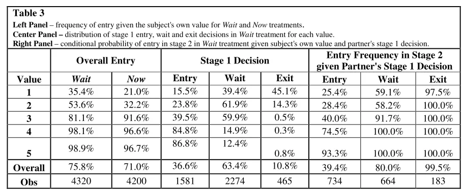
Surprisingly and counter to our conjecture, a comparison of treatments according to the
overall percentage of entry (see the left panel of Table 3) reveals a higher percentage of
entry decisions in Wait (75.8%) than in Now (71.0%). Subjects are 14 percentage points
(hereafter "p.p.") more likely to enter on a 1 in Wait (35.4%) than in Now (21.0%). This
gap between treatments grows to 21 p.p. on the value of 2. In fact, higher entry in Wait
holds for all values except 3. If we treat each subject's fraction of decisions corresponding
to enter as the unit of observation, then the non-parametric Wilcoxon-Mann-Whitney test
rejects the equality of the entry frequency distributions (z=-1.99, p=0.047, n=142).
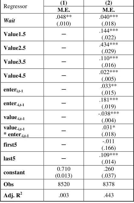
In Table 4, we report the estimates from two linear probability models on subject i's
decision to enter in period t.7 Standard errors are clustered by subject, taking into account possible correlation in the error terms across periods of play. Regression (1) includes only
an indicator variable for the Wait treatment. The highly significant coefficient of 0.048
(p=0.026) confirms the significant difference between entry frequencies in Wait and Now.
Despite a series of controls for game variables and lagged play in regression (2), the
difference in entry frequency across treatments remains around 4 p.p. and highly
significant (p=0.026).
The indicator variable Value1.5 equals 1 if subject i's period t value is 2, 3, 4 or 5
and 0 if it is 1. Similarly, Value2.5 equals 1 if subject i's period t value is 3, 4 or 5 and 0
if it is 1 or 2 and so forth for Value3.5 and Value4.5. The estimated coefficients on
Value1.5, Value2.5, Value3.5 and Value4.5 reflect the marginal propensity to enter on a
2, 3, 4 or 5, respectively. The highly significant coefficients reveal that subjects were
7
increasingly more likely to enter on each additional value. The likelihood of entering on a
3 is a whopping 43 p.p. higher than it is on a 2. The regression also reveals that the
subject's previous period entry and especially that of his partner are associated with a
higher likelihood of entry in the current period. Subjects also appear to take into account
their partner's previous-period value in a conciliatory manner: for every additional point
the partner received last period, the subject is four p.p. less likely to enter this period.
Finally, the highly significant coefficient of 0.11 on the indicator variable for play in the
final five rounds attests to a modest breakdown in cooperation as the known terminal
period approaches. No significant difference in the propensity to enter is observed
between the first five rounds (or similarly for the first 10 rounds (not shown)) and the
middle 50 (or middle 45) rounds.
4.2 Profits
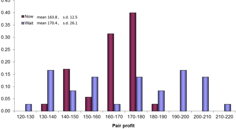
Higher entry in Wait may lead us to expect lower profits than in Now. However, the mean
pair profit of 170.4 in Wait actually exceeds that of 163.8 in Now. If we express the mean
pair profit by treatment as a percentage of the full-information efficient outcome by
which only the high-value player enters (in the case of ties only one player enters) using
the actual distribution of values drawn over the 60 rounds, Wait subjects reach 73.1% of
this first-best social optimum on average, which is significantly and nearly three p.p.
higher than the 70.3% obtained in Now (Wilcoxon-Mann-Whitney z=-1.81, p = 0.07).
Both percentages greatly exceed the 52.6% earned by Nash play, attesting to the
relatively high levels of cooperation achieved in both treatments.
4.3 Outcomes and the use of waiting to aid in coordination
How did subjects in Wait manage to earn higher profits despite such seemingly high
levels of entry? Table 5 categorizes all game outcomes according to whether only the
player with the higher value entered (efficient cooperation), only the low-value player
entered (inefficient cooperation), both entered (double entry) or neither entered (double
exit). The largest difference between the two treatments is that double exit (the
lowest-payoff outcome) is six p.p. higher in Now (8.9%) than in Wait (2.9%). The missing six
40.2% in Now to 42.5% in Wait). A chi-square test of proportions shows that the
differences in percentages of the outcomes between the treatments are highly significant
(χ2=78.4, d.f.=3, p<0.01).
Increased efficient cooperation in Wait is the result of lower-value subjects waiting
in stage 1 and, after observing their partner enter in stage 1, exiting in stage 2. The center
panel of Table 3 shows that waiting was the modal stage-one decision for values 2 and 3,
comprising about 60% of the decisions in both cases. Waiting constitutes another 40% of
stage-one decisions when the subject received a 1; although, exit – the choice which
guarantees against double entry – is the modal choice (45%). By contrast, exit occurs less
than 1% of the time on the highest values of 4 and 5, with waiting accounting for between
12% and 15% of decisions and entering amounting to 85%-87%. In short, subjects tend to
wait or exit on the lowest value of 1, wait on values 2 and 3, and enter with a 4 or 5.
The right panel of Table 3 shows that subjects follow through on their first-stage
waiting decision to avoid double exit and, to a lesser extent, double entry in the second
stage. After waiting in stage 1, subjects enter nearly 100% of the time if their partners
exited in stage 1 (avoid double exit). Less emphatically, stage-two exit frequencies vary
from a mere 7% with a value of 5 to 75% with a value of 1 after observing the partner
entered in stage 1 (avoid double entry). When both players wait, the resulting subgameis
strategically equivalent to Now. However, having seen the partner’s decision to wait
allows the player to update his beliefs about the other’s value. Based upon the observed
waiting frequencies, the chance that the partner has a value of 4 or 5 is reduced from 40%
(ex ante) to 14.5% (observed). Updating their beliefs about their partners' values
accordingly provides a possible rationale for entering on lower values and may partially
account for the higher entry frequencies observed on values 1 and 2 in Wait than in Now.
The above stage-two entry percentages present a puzzle. They range from 25% to an
alarming 93% after the partner entered in stage 1. Waiting can be beneficial when used to
gather information to facilitate efficient coordination and a higher payoff for the pair. Yet
entry after seeing the partner enter implies waiting was not adopted to avoid double entry.
Alternatively, perhaps waiting was invoked to punish partners who entered while
partner wait than after seeing him enter casts doubt on this punishment explanation.8 Instead, a subject who enters after seeing a partner enter seems intent on entering
regardless of any information received after stage 1. Given the intention to enter, why
wait rather than enter in the first place? The likely answer is that waiting may be
perceived as a less egregious action than directly entering. Thus, by first waiting, the
subject wishes to appear cooperative to his partner. Later we will examine further this
strategy and its success.
4.4 Distribution of Pair Profits
As a prelude to assessing the success of various strategies, let us take a closer look at the
distribution of profits across treatments, currently masked by the simple comparison of
mean profits discussed in Section 4.2. Figure 1 reveals a relatively diffuse distribution of
pair profits in Wait compared to the highly concentrated distribution in Now. The
distribution of pair profits in Wait resembles a uniform distribution, whereas 71.4% of the
pairs in Now earned profits in the narrow range of 160 to 180. In fact, the highest pair
profit was 181, meaning that not a single pair appears in any of the three highest profit
categories. Contrast this with a highest pair profit of 215.7 in Wait and 31% of the pairs
that placed in the three highest profit categories. At the other extreme, the four lowest
earning pairs in the experiment with pair profits of 125, 131, 131, 132 all originate from
Wait, below the lowest pair profit in Now of 135.
The upshot of these differences is that the distributions of pairs' profits intersect near
50%. That is, about half of the pairs in Wait earned lower profits than pairs in Now. To
demonstrate the robustness of the intersection between the two profit distributions,
avoiding it would require removing the nine pairs with the lowest profits from Wait (out
of 36 pairs in total).
8
Why do so many pairs in Wait earn low profits, despite the better conditions for
coordination? To address this question, we analyze in the next two subsections how the
behavior of the low-profit subjects in Wait differs from that of the high-profit subjects.
4.5 Individual Strategy Inference
Recall from Section 3 that there are 21 possible monotonic cutoff strategies in stage 1
that condition on the subject's value. For each subject we compare the ability of each of
the 21 monotonic cutoff strategies in Table 2 and the alternating strategy to classify
correctly subjects’ decisions in stage 1. The strategy that minimizes the number of errors
in classifying the subject’s observed decisions is deemed the strategy the subject most
likely employed. Table 6 presents the distribution of these best-fit strategies for stage 1 of
Wait (left panel) and for Now (right panel).9 For each strategy we denote the number of subjects that employ the strategy (column 2)10 and the mean number of errors (deviations from the strategy) by those who employed it (column 3).
In Wait, 86.5% of the subjects employ strategies that involve waiting. The remaining
13.5% of subjects simply enter on all values (7.6%) or enter on values 2-5 and exit on 1
(5.9%). Capturing 21/72 subjects, the strategy 1(23)45 is the most widely employed. It is
also the second most jointly profitable symmetric strategy, as evidenced by the high
realized mean profit of 95.6 (column 4 of Table 6) earned by its adopters. The strategy of
(123)45 is the second most widely used strategy with 12.5/72 subjects using it. These two
strategies differ only in that 1(23)45 dictates exiting on the value of 1 while (123)45 calls
for waiting. The latter choice to wait leads to lower mean profits of 82.9. One lone
subject employed the joint profit-maximizing symmetric strategy of 1(234)5, while no
pair was found to play any of the asymmetric strategic pairs that jointly earn more than
1(234)5. Nor did any pairs adopt the payoff-inferior alternating strategy in Wait.
9
The inferred strategies are based on rounds 6-55 and thus exclude decisions in the ten periods possibly influenced by learning in the initial rounds and the endgame effect. The distributions of best-fit strategies are highly robust to other ranges of included periods, such as all 60 rounds, the first 50 or 55 rounds and the last 50 rounds.
10
The subject's profit along with that of his partner (column 5) attest to the pairs' degree
of cooperation. Paired partners in which at least one pair member followed the strategy
1(23)45 earned similarly high profits, implying a high level of cooperation. Those who
followed the strategy 1(23)45 recorded the fewest deviations from their inferred
strategy.11 Tracking this strategy to stage 2, subjects on the whole appear to be playing the strategy 1(2/3)45 (wait and exit with value 2, wait and enter with value 3 when the
partner also waited).
The right panel of Table 6 displays the best-fit strategies for subjects in the Now
treatment. Forty-four of 70 (62%) subjects employed the strategy 12()345, meaning they
exited on values 1 and 2, and entered on values 3, 4 and 5. In striking contrast, not a
single subject utilized this strategy in Wait in which the waiting option is available. Only
two pairs of subjects used the alternating strategy despite it being the most profitable
strategy in this treatment.
The dominant strategy of "always enter" was employed by twice as many subjects in
Now as in Wait (15% and 7.6% respectively). In Wait, the mean subject profit for the
strategy ()12345 (always enter) of only 65.0 is almost 50% below the mean subject profit
for 1(23)45 of 95.6. In Now, the mean subject profit for the always enter strategy of 76.4
is 11% below the mean profit of 84.5 for socially optimal cutoff strategy of 12()345 and
12% below the mean profit of 85.3 from alternating. Cooperative subjects earn
substantially more than uncooperative subjects, especially in the Wait treatment.
4.6 Behavior of Low-Profit Subjects in
Wait
Overall, the possible sources of low profits in Wait are inefficient cooperation, double
exit and double entry outcomes. Yet, we saw that inefficient cooperation and double
11
Overall, the error rates are low for most strategies, thereby attesting to the effectiveness of this simple technique in capturing subjects' behavior. Of the 3600 decisions made by the 72 subjects in Wait between rounds 6-55, 3132 (or 87%) correspond to the best-fit strategy inferred for each subject compared to 3220 out of the 3500 (or 92%) decisions made by the 70 subjects in Now. With a binary decision in Now, the percentage of errors in Now is naturally lower than in Wait. The addition of the waiting option in Wait
exiting occur with strikingly low frequency in Wait (1.6% and 2.9% respectively
according to Table 4). Double entry, on the contrary, accounts for 51% of the outcomes,
57.3% of which arise from both subjects entering in stage 1, 18.2% from both subjects
entering in stage 2, and a troubling 24.5% from subjects entering in different stages. The
percentages of double entry in stage 2 and especially entry in different stages are
distressingly high and attest to uncooperative decisions.
An analysis of the second-stage decisions shows that subjects do not necessarily
choose the action opposite to their partner's first-stage action. When paired subjects both
wait in stage 1, Table 7 reveals that they tend to enter in stage 2 when their value is 5 or 4
(and in most cases when their value is 3). When their value is 1 or 2, the likelihood of
entry differs dramatically between subjects and is highly negatively correlated with the
degree of cooperation and profits achieved by the pair. For example, we see from Table 7
that for the three lowest pair profit categories (i.e., profits below 180), entry is the modal
stage-two decision after the partner waited in stage 1 for all five values. By contrast, exit
is the modal decision on a value of 1 for the second-highest profit category and on values
1 and 2 for the highest profit category.
The differences in entry percentages across profit categories for a given value are
even more stark conditional on the partner entering in stage 1 (Table 8). Despite the
partner having already visibly entered in stage 1, subject pairs in the lowest profit
category nonetheless enter with a frequency of 66.7% on a value of 1, increasing to 100%
on values 4 and 5. Moving across the table, these entry frequencies drop dramatically for
the second-highest and highest profit categories; in neither of these profit categories did
anyone enter on a value of 1. No entry also holds for a value of 2 for the highest category.
In fact, among the highest profit pairs, the entry frequency increases to only 11.1% on a
value of 4.
Moreover, Tables 7 and 8 both attest to sharp increases in the entry percentage after
waiting as the value increases for the two highest profit categories of 180-199 and
200-220. However, for the three lower profit categories, entry percentages begin much higher
and rise more modestly as the value increases. In other words, successful subject pairs
condition their second-stage entry decision on their value and their partners' first-stage
The individual strategy analysis allows us to examine this behavior in more detail.
Although, as already noted, fewer subjects employed "always enter" in Wait (5.5 subjects
versus 10.5 in Now), another 5.5 subjects played "always wait". We conjectured that its
likely reason is to feign cooperative behavior. Indeed, looking at the second-to-last
column of Table 6, those classified as “always wait” (12345) entered an astonishing 98%
of the time compared to 89% entry by “always enter” subjects in Wait and 87% by
“always enter” subjects in Now. That is, the always wait subjects are wholly
uncooperative – even more so than those who play always enter. The availability of the
waiting option seems to attract the least cooperative types and, under the guise of waiting
to decide, entices them to behave even more uncooperatively than they would in the
absence of this option.
Now the natural question to ask is: were they successful in their attempt to deceive
their partners? The last column of Table 6 reveals that their uncooperativeness was
reciprocated with entry of 90% by their partners. This compares with entry of 85% by
partners paired against “always enter” in Wait and 82% against “always enter” in Now.
Hence, subjects' attempt to deceive was foiled leading to low profits for themselves and
the pair overall. The addition of the waiting option failed to conceal uncooperativeness
whether in the form of always enter or always wait followed by entry.
5
Conclusions
This paper examines experimentally how the option of waiting affects cooperation.
Although subjects entered more often in the Wait treatment for almost all entry values,
the timing of the entry enabled paired players to achieve a higher degree of cooperation
and ultimately higher profits in Wait. Thus, the ability to time decisions plays a crucial
role in resolving in cooperative dilemmas.
Yet, a closer look at the distribution of subjects' profits reveals that while profits in
Wait were higher on average, nearly half of the subjects in this treatment earned less than
in Now. The dark side of the waiting option is that this tool designed to enhance
cooperation helps only those with a desire to cooperate: selfish individuals exploit the
References
Angrist, J. D., Pischke, J.-S. 2009. Mostly Harmless Econometrics: An Empiricist’s Companion, Princeton University Press.
Cason, T. N., Lau, S.-H. P., Mui, V.-L. 2012. "Learning, teaching, and turn-taking in the repeated assignment game", Economic Theory.
Chamley, C., Gale, D. 1994. "Information revelation and strategic delay in a model of investment", Econometrica 62, 1065-1085.
Dietz, T., Ostrom, E., Stern, P.C. 2003. "The struggle to govern the commons", Science 302(5652), 1907-1912.
Engelmann, D., and Grimm, V. 2011. “Mechanisms for Efficient Voting with Private Information about Preferences”, Economic Journal 122(563), 1010-1041.
Fonseca, M. A., Normann, H.-T. 2008. "Mergers, Asymmetries and Collusion: Experimental Evidence", Economic Journal 118(527), 387-400.
Gul, F., Lundholm, R. 1995. "Endogenous timing and the clustering of agents' decisions", Journal of Political Economy 103, 1039-1066.
Hamilton, J. H., Slutsky, S. M. 1990. “Endogenous timing in duopoly games: Stackelberg or Cournot equilibria”, Games and Economic Behavior 2, 29–46.
Huck, S., Muller, W., Normann, H.-T. 2001. “Stackelberg beats Cournot – on collusion and efficiency in experimental markets”, Economic Journal 111 749–766.
Huck, S., Muller, W., Normann, H.-T. 2002. "To commit or not to commit: endogenous timing in experimental duopoly", Games and Economic Behavior 38, 240–264.
Kaplan, T., Ruffle, B. J. 2012. "Which way to cooperate", Economic Journal 122(563), 1042-1068.
Ostrom, E. 2009. Understanding institutional diversity. Princeton University Press.
Ostrom, E., Walker, J., and Gardner, R. 1992. "Covenants with and without a sword: Self-governance is possible", American Political Science Review, 86(2), 404-417.
Potters, J., Sefton, M., Vesterlund, L. 2005. "After you - endogenous sequencing in voluntary contribution games", Journal of Public Economics 89(8) 1399-1419.
Ziegelmeyer, A., Boun My, K., Vergnaud, J., Willinger, M. 2005. "Strategic delay and rational imitation in the laboratory", working paper, Max Planck Institute of Economics.
[image:18.595.130.467.219.340.2]Zillante, A. 2011. “Recognizing and Playing Turn Taking Strategies” working paper.
Table 1 – Payoff Matrix
Player with value B
stage Stage 1 enter exit wait Stage 2 - - enter exit
Player with value A
enter - 1/3A, 1/3B A,0 1/3A, 1/3B A,0 exit - 0,B 0,0 0,B 0,0
wait enter 1/3A, 1/3B A,0 1/3A, 1/3B A,0 exit 0,B 0,0 0,B 0,0
Table 3
Left Panel – frequency of entry given the subject's own value for Wait and Now treatments.
Center Panel – distribution of stage 1 entry, wait and exit decisions in Wait treatment for each value.
Right Panel – conditional probability of entry in stage 2 in Wait treatment given subject's own value and partner's stage 1 decision.
Overall Entry Stage 1 Decision
Entry Frequency in Stage 2 given Partner's Stage 1 Decision Value Wait Now Entry Wait Exit Entry Wait Exit
1 35.4% 21.0% 15.5% 39.4% 45.1% 25.4% 59.1% 97.5%
2 53.6% 32.2% 23.8% 61.9% 14.3% 28.4% 58.2% 100.0%
3 81.1% 91.6% 39.5% 59.9% 0.5% 40.0% 91.7% 100.0%
4 98.1% 96.6% 84.8% 14.9% 0.3% 74.5% 100.0% 100.0%
5 98.9% 96.7%
86.8% 12.4%
0.8% 93.3% 100.0% 100.0%
Overall 75.8% 71.0% 36.6% 63.4% 10.8% 39.4% 80.0% 99.5%
[image:18.595.68.523.392.580.2]Table 2
The joint expected payoffs for any pair of strategies among 21 monotonicstrategies and alternating (Wait treatment)
Player 2
1 2 3 4 5 6 7 8 9 10 11 12 13 14 15 16 17 18 19 20 21 22
12345() 1234(5) 1234()5 123(45) 123(4)5 123()45 12(345) 12(34)5 12(3)45 12()345 1(2345) 1(234)5 1(23)45 1(2)345 1()2345 [12345] (1234)5 (123)45 (12)345 (1)2345 ()12345 Alternate
P
la
y
e
r
1
1 12345() 0.00 1.00 1.00 1.80 1.80 1.80 2.40 2.40 2.40 2.40 2.80 2.80 2.80 2.80 2.80 3.00 3.00 3.00 3.00 3.00 3.00 1.50
2 1234(5) 1.00 1.80 1.80 2.42 2.42 2.40 2.86 2.86 2.84 2.80 3.12 2.92 3.10 3.06 3.00 3.20 3.20 3.18 3.28 3.14 3.00 2.00
3 1234()5 1.00 1.80 1.73 2.44 2.37 2.29 2.92 2.85 2.77 2.68 3.24 3.17 3.09 3.00 2.89 3.40 3.33 3.25 3.16 3.05 2.93 1.97
4 123(45) 1.80 2.42 2.44 2.88 2.9 2.88 3.18 3.20 3.18 3.12 3.32 3.34 3.32 3.26 3.16 3.30 3.32 3.30 3.24 3.14 3.00 2.40
5 123(4)5 1.80 2.42 2.37 2.90 2.85 2.77 3.24 3.19 3.11 3.00 3.44 3.39 3.21 3.20 3.05 3.50 3.45 3.37 3.26 3.11 2.93 2.37
6 123()45 1.80 2.40 2.29 2.88 2.77 2.64 3.24 3.13 3.00 2.84 3.48 3.37 3.24 3.08 2.89 3.60 3.49 3.36 3.20 3.01 2.80 2.30
7 12(345) 2.40 2.86 2.92 3.18 3.24 3.24 3.36 3.42 3.42 3.36 3.40 3.46 3.46 3.40 3.28 3.30 3.36 3.36 3.30 3.18 3.00 2.70
8 12(34)5 2.40 2.86 2.85 3.20 3.19 3.13 3.42 3.41 3.35 3.24 3.52 3.51 3.45 3.34 3.17 3.50 3.49 3.43 3.32 3.31 2.93 2.67
9 12(3)45 2.40 2.84 2.77 3.18 3.11 3.00 3.42 3.35 3.24 3.08 3.56 3.49 3.38 3.22 3.01 3.60 3.53 3.42 3.26 3.05 2.80 2.60
10 12()345 2.40 2.80 2.68 3.12 3.00 2.84 3.36 3.24 3.08 2.88 3.52 3.40 3.24 3.04 2.80 3.60 3.48 3.32 3.12 2.88 2.60 2.50
11 1(2345) 2.80 3.12 3.24 3.32 3.44 3.48 3.40 3.52 3.56 3.52 2.80 3.48 3.56 3.48 3.36 3.20 3.32 3.36 3.32 3.20 3.00 2.90
12 1(234)5 2.80 2.92 3.17 3.34 3.39 3.37 3.46 3.51 3.49 3.40 3.48 3.53 3.51 3.42 3.25 3.40 3.45 3.43 3.46 3.17 2.93 2.87
13 1(23)45 2.80 3.10 3.09 3.32 3.21 3.24 3.46 3.45 3.38 3.24 3.56 3.51 3.44 3.30 3.09 3.50 3.49 3.42 3.28 3.07 2.80 2.80
14 1(2)345 2.80 3.06 3.00 3.26 3.20 3.08 3.40 3.34 3.22 3.04 3.48 3.42 3.30 3.12 2.88 3.50 3.44 3.32 3.14 2.90 2.60 2.70
15 1()2345 2.80 3.00 2.89 3.16 3.05 2.89 3.28 3.17 3.01 2.80 3.36 3.25 3.09 2.88 2.61 3.40 3.29 3.13 2.92 2.65 2.33 2.57
16 (12345) 3.00 3.20 3.40 3.30 3.50 3.60 3.30 3.50 3.60 3.60 3.20 3.40 3.50 3.50 3.40 3.00 3.20 3.30 3.30 3.20 3.00 3.00
17 (1234)5 3.00 3.20 3.33 3.32 3.45 3.49 3.36 3.49 3.53 3.48 3.32 3.45 3.49 3.44 3.29 3.20 3.33 3.37 3.32 3.17 2.93 2.97
18 (123)45 3.00 3.18 3.25 3.30 3.37 3.36 3.36 3.43 3.42 3.32 3.36 3.43 3.42 3.32 3.13 3.30 3.37 3.36 3.34 3.07 2.80 2.90
19 (12)345 3.00 3.28 3.16 3.24 3.26 3.20 3.30 3.32 3.26 3.12 3.32 3.46 3.28 3.14 2.92 3.30 3.32 3.34 3.12 2.90 2.60 2.80
20 (1)2345 3.00 3.14 3.05 3.14 3.11 3.01 3.18 3.31 3.05 2.88 3.20 3.17 3.07 2.90 2.65 3.20 3.17 3.07 2.90 2.65 2.33 2.67
21 ()12345 3.00 3.00 2.93 3.00 2.93 2.80 3.00 2.93 2.80 2.60 3.00 2.93 2.80 2.60 2.33 3.00 2.93 2.80 2.60 2.33 2.00 2.50
22 Alternate 1.50 2.00 1.97 2.40 2.37 2.30 2.70 2.67 2.60 2.50 2.90 2.87 2.80 2.70 2.57 3.00 2.97 2.90 2.80 2.67 2.50 3.00
Table 4
Linear Probability Model on overall decision to enter
Regressor (1) (2)
M.E. M.E.
Wait .048**
(.010)
.040*** (.018)
Value1.5 ─ .144***
(.022)
Value2.5 ─ .434***
(.029)
Value3.5 ─ .110***
(.016)
Value4.5 ─ .022***
(.005)
enteri,t-1 ─
.033** (.015)
enter-i,t-1 ─
.181*** (.019)
value-i,t-1 ─
-.038*** (.004)
value-i,t-1
* enter-i,t-1
─ .031*
(.018)
first5 ─ -.011
(.166)
last5 ─ .109***
(.014)
constant 0.710
(0.013)
.260 (.037)
Obs 8520 8378
Adj. R2 .003 .443
Table 5
Percentage of outcomes by treatment
Outcome Now Wait
efficient cooperation 37.3% 40.9% inefficient cooperation 2.9% 1.6%
double entry 51.0% 54.6%
double exit 8.9% 2.9%
Total 100.0% 100.0%
Double entry - both subjects enter Double exit - both subjects exit
Efficient cooperation – the subject with the higher value enters, while the other subject exits
Inefficient cooperation - the subject with the lower value enters, while the other subject exits
Dependent variable - enterit equals 1
if subject i entered in period t and equals 0 if subject exited in period t
Wait equals 1 if observation is from
Wait and 0 if from Now
Value1.5equals 1 if subject i’s period
t value is 2, 3, 4 or 5 and equals 0 if value is 1. Similarly, Value2.5 equals 1 for values 3, 4 or 5 and 0 otherwise, and so forth for Value3.5 and
Value4.5
enteri,t-1, enter-i,t-1 are subject’s and
his partner's previous period entry decisions
value-i,t-1 is partner's previous period
value (from 1 to 5)
value-i,t-1*enter-i,t-1 is interaction term
between partner's previous period value and entry decision
first5 equals 1 if rounds 1-5, last5
equals 1 if rounds 56-60, 0 otherwise
[image:20.595.190.410.532.715.2]Table 6
Distribution of strategies, mean own and partner's mean profit and mean fraction of errors by strategy and treatment, rounds range 6-55
Wait Now
Strategy Number who played strategy Fraction of errors Mean profit Mean profit of partner Entry percent (after both stages) Partner entry percent (after both stages) Number who played strategy Fraction of errors Mean profit Mean profit of partner Entry percent Partner entry percent in v o lv e w ai ti n g
12 (3) 45 7 .07 96 93.4 62.9% 66.0% - - - - 1 (2345) 0.5 .36 63.7 75.7 88.3% 98.3% - - - - 1 (234) 5 1 .08 92 123.7 45.0% 51.7% - - - - 1 (23) 45 21 .08 95.6 92.6 63.9% 65.4% - - - - 1 (2) 345 0.25 .20 81.3 82.3 73.3% 76.7% - - - - (12345) 5.5 .26 69 64.5 97.8% 90.0% - - - - (1234) 5 1 .42 82.7 60.7 96.7% 73.3% - - - - (123) 45 12.5 .14 82.9 80.1 79.4% 74.4% - - - - (12) 345 8.75 .15 82.2 79.4 82.0% 81.0% - - - - (1) 2345 4.75 .10 74.2 75.5 86.4% 85.3% - - - -
d o n o t in v o lv e w ai ti n g
() 12345 5.5 .18 65 70.8 88.6% 85.5% 10.5 .13 76.4 70.8 87.3% 81.8% 1 () 2345 4.25 .15 76.4 80.3 84.2% 89.6% 11 .10 75.5 77.3 80.0% 82.1%
12 () 345 - - - - 44 .5 84.5 85.3 66.5% 67.6%
123 () 45 - - - - 0.5 .16 77.7 87.3 56.7% 60.0%
1234 () 5 - - - -
12345 () - - - -
alternating - - - - 4 .14 85.3 85.3 55.8% 55.8%
Table 7
Percentage of entry decisions in stage 2 (Wait), conditional on partner waiting in stage 1, by profit category and value
Value / Profit category
120-139 140-159 160-179 180-199 200-220 Overall
Perc. Obs. Perc. Obs. Perc. Obs. Perc. Obs. Perc. Obs. 1 86.7% 45 54.5% 33 54.8% 31 25.0% 24 25.0% 4 59.1% 2 87.5% 40 90.0% 20 88.2% 17 50.9% 55 30.3% 33 58.2% 3 98.2% 55 100.0% 24 100.0% 14 92.8% 83 77.4% 53 91.7% 4 100.0% 46 100.0% 10 100.0% 4 100.0% 8 100.0% 3 100.0% 5 100.0% 42 100.0% 8 100.0% 6 100.0% 5 100.0% 1 100.0% Number
[image:22.595.116.497.556.765.2]of pairs 7 8 6 9 6 36
Table 8
Percentage of entry decisions in stage 2 (Wait), conditional on partner entering in stage 1, by profit category and value
Value / Profit category
120-139 140-159 160-179 180-199 200-220 Overall
Perc. Obs. Perc. Obs. Perc. Obs. Perc. Obs. Perc. Obs. 1 66.7% 21 25.5% 47 12.9% 31 0.0% 3 0.0% 7 27.5% 2 93.9% 33 67.5% 40 15.7% 51 6.7% 30 0.0% 44 34.3% 3 93.1% 29 90.3% 31 64.5% 31 24.1% 29 4.5% 66 45.7% 4 100.0% 19 80.0% 15 100.0% 6 50.0% 2 11.1% 9 76.5% 5 100.0% 27 88.9% 9 100.0% 3 100.0% 1 60.0% 5 93.3% Number
of pairs 7 8 6 9 6 36
Appendix A: Monotonic Strategies
Proposition: The pair’s joint profits are maximized by each pair member using a
monotonic strategy in the first stage of the two-stage. This will never entail the
degenerate case of one player always entering and the other always exiting.
Proof: More general than our simple game, suppose that each player receives a randomly drawn integer between a and b inclusive where the probability of receiving a number x is Пx (where Пx > 0 and ∑x€{a...b} Пx = 1). By exiting a player receives zero
and entering he receives his number if the other player exits, but receives some function f(x) increasing in his number, x, if both enter (in stage 1 or in stage 2). We assume that f(x) is strictly less than his number x (and f’(x)<1); hence entry imposes a negative externality on the other player. We also assume that if it is profitable for a player to enter alone (that is, his value is greater than zero), then it is also profitable for him to enter when his partner enters (f > 0 for values greater than zero).
The cooperative solution is given by the pair of strategies that maximizes the sum of the players’ expected payoffs. If the player waited in stage 1, we assume he will enter and receive his number if his partner exited in stage 1, and he will exit and receive zero if his partner entered in stage 1.
Suppose the partner enters with probability p(y) and waits with probability t(y) when his number is y. The value of both waiting and optimally cooperating in the second stage is z(x,y), which is weakly increasing in x and weakly decreasing in y (from the cutoff strategies found in the one-stage game in Kaplan and Ruffle, 2012). The joint expected payoff to entering in stage 1 with number x is,
∏
y{
x
(1
−
p
(
y
)
−
t
(
y
))
+
p
(
y
)(
f
(
x
)
+
f
(
y
))
+
x
⋅
t
(
y
)}
y∈{a,b}
∑
The joint expected payoff to exiting out in stage 1 withnumber x is
∏
y{
yp
(
y
)
+
y
⋅
t
(
y
)}
y∈{a,b}
∑
.The joint expected payoff to waiting in stage 1 with number x is
∏
y{
x
(1
−
p
(
y
)
−
t
(
y
))
+
yp
(
y
)
+
t
(
y
)
z
(
x
,
y
)
y∈{a,b}
∑
}
.First, note that ∑ ∈{ , } ( )(z(x + 1, y) − z(x, y)) ≤ ∑ ∈{ , } ( ). If
∑ ∈{ , } ( )(z(x + 1, y) − z(x, y)) > ∑ ∈{ , } ( ), then we can use the same
due to player 1 receiving x or f(x) when the second player waits must be r*x+q*f(x) where r+q≤1, hence the derivative r+qf’(x)≤1. This would contradict the assumption that z(x,y) entails optimal cooperation.
We now see that the cooperative solution entails monotonic strategies. This is because if the joint expected payoff to entering is greater than the joint expected payoff to waiting for x, then it also holds for any value greater than x. And likewise if the joint expected payoff to waiting exceeds the joint expected payoff to exiting.
We still have to worry about the case of indifference between waiting and entering for several values of x. Indifference occurs only if the partner always stays out. The pair then earns the same whether the player enters or waits and then enters. In a repeated game, one player always exiting and the other always entering can take the form of alternating. As long as the upper bound of one player L's range of numbers strictly exceeds the lower bound of his partner H's range of numbers (and vice-versa), always exiting and alternating in the repeated game can never be socially optimal since the player always exiting (player L) can wait with his highest number and the player always entering (player H) can wait with any number strictly below that number. Whenever both players wait, player L enters and player H exits in stage 2 to obtain a higher joint payoff than from player L always exiting.
Appendix B: Instructions Sheets
Wait Treatment - Instructions Sheet
Welcome
The experiment in which you will participate involves the study of decision-making. If you follow the instructions carefully and make wise decisions, you may earn a considerable amount of money. Your earnings depend on your decisions. All of your decisions will remain anonymous and will be collected through a computer network. Your choices are to be made at the computer at which you are seated. Your earnings will be revealed to you as they accumulate during the course of the experiment. Your total earnings from the experiment will be paid to you, in cash, at the end of the experiment.
You are requested not to talk to one another at any time during the experiment. If you have any questions, raise your hand and a monitor will assist you. It is important that you understand the instructions. Misunderstandings can result in lower earnings. Finally, we ask that even after the experiment is over you not discuss the details of this experiment with anyone.
Your information
At the beginning of each round, you and the person with whom you are paired each receives a randomly drawn number between 1 and 5 inclusive. You will see your number, and learn the other person's number only after the round ends.
Decision Stage 1
After you've seen your number and the other person has seen his number, each of you must decide separately between one of three actions: enter, exit or wait.
Decision Stage 2
If you choose to wait in stage 1 and the other person chooses to enter or exit, you will see his decision after stage 1 ends. Then in stage 2 you must decide between one of two actions: enter or exit.
If you choose to enter or exit in stage 1 and the other person chooses to wait, he will see your decision after stage 1 ends. Then in stage 2 the other person must decide between one of two actions: enter or exit.
If you both choose to wait in stage 1, in stage 2 each of you must decide separately between one of two actions: enter or exit.
In other words, each person must ultimately decide whether to enter or exit. Each person may decide to enter or exit in stage 1 or wait until stage 2 to decide whether to enter or exit after observing the other person's decision in stage 1.
Round Profit
At the end of each round, your number, your decision, and the other person’s decision determine your round profit in the following way.
- If you both chose to exit (in either stage 1 or stage 2), then you both receive zero points.
- If you chose to exit (in either stage 1 or stage 2) and the other person chose to enter (in either stage 1 or stage 2), then you receive zero points and the other person receives points equal to his number.
- If you chose to enter (in either stage 1 or stage 2) and the other person chose to exit (in stage 1 or stage 2), you receive points equal to your number and the other person receives zero points.
- If you both chose to enter (in stage 1 or stage 2), then you receive points equal to one-third of your number and the other person receives points equal to one-third of his number.
The table below summarizes the payoff structure. Suppose you receive a number, x, and the other person receives a number, y. The round profits for each of the given pair of decisions are indicated in the table below. The number preceding the comma refers to your round profit; the number after the comma is the other person’s round profit.
After you have both made your decisions for the round, you will see the amount of points you have earned for the round, the other person's number and the other person’s decision. Please record these results from each round in your Personal Record Sheets. When you are ready to begin the next round, press Continue.
Enter
(stage 1 or 2)
Exit
(stage 1 or 2)
You
Enter
(stage 1 or 2) x/3, y/3 x, 0
Exit
(stage 1 or 2) 0, y 0, 0
Total Payment
Each round follows this same sequence of events. At the end of the experiment, you will be paid your accumulated earnings from the experiment in cash. Each point earned in the experiment is equivalent to 0.9 shekels. While the earnings are being counted, you will be prompted to complete a questionnaire.
Prior to the beginning of the experiment, you will partake in five practice rounds. The profits earned in these practice rounds will not be included in your payment. The rules of the practice rounds are otherwise identical to those of the experiment in which you will participate. The purpose of the practice rounds is to familiarize you with the rules of the experiment and the computer interface. Note well that for the purpose of the practice rounds, you will be paired with a different person from the actual experiment.
Thank you for your participation
Now Treatment – Instructions Sheet
Welcome
The experiment in which you will participate involves the study of decision-making. If you follow the instructions carefully and make wise decisions, you may earn a considerable amount of money. Your earnings depend on your decisions. All of your decisions will remain anonymous and will be collected through a computer network. Your choices are to be made at the computer at which you are seated. Your earnings will be revealed to you as they accumulate during the course of the experiment. Your total earnings from the experiment will be paid to you, in cash, at the end of the experiment.
You are requested not to talk to one another at any time during the experiment. If you have any questions, raise your hand and a monitor will assist you. It is important that you understand the instructions. Misunderstandings can result in lower earnings. Finally, we ask that even after the experiment is over you not discuss the details of this experiment with anyone.
There are several experiments of the same type taking place at the same time in this room.
This experiment consists of 60 rounds. You will be paired with another anonymous person. This person will remain the same for all 60 rounds.
Your information
At the beginning of each round, you and the person with whom you are paired each receives a randomly drawn number between 1 and 5 inclusive. You will see your number, and learn the other person's number only after the round ends.
After you've seen your number and the other person has seen his number, each of you must decide separately between one of two actions: enter or exit.
Round Profit
At the end of each round, your number, your decision, and the other person’s decision determine your round profit in the following way.
- If you both chose to exit, then you both receive zero points.
- If you chose to exit and the other person chose to enter, then you receive zero points and the other person receives points equal to his number.
- If you chose to enter and the other person chose to exit, you receive points equal to your number and the other person receives zero points.
- If you both chose to enter, then you receive points equal to one-third of your number and the other person receives points equal to one-third of his number.
The table below summarizes the payoff structure. Suppose you receive a number, x, and the other person receives a number, y. The round profits for each of the given pair of decisions are indicated in the table below. The number preceding the comma refers to your round profit; the number after the comma is the other person’s round profit.
Other Person
Enter Exit
You Enter x/3, y/3 x, 0
Exit 0, y 0, 0
After you have both made your decisions for the round, you will see the amount of points you have earned for the round and the other person’s decision and number. Please record these results from each round in your Personal Record Sheets. When you are ready to begin the next round, press Continue.
Total Payment
Each round follows this same sequence of events. At the end of the experiment, you will be paid your accumulated earnings from the experiment in cash. Each point earned in the experiment is equivalent to 0.9 shekels. While the earnings are being counted, you will be prompted to complete a questionnaire.
Prior to the beginning of the experiment, you will partake in five practice rounds. The profits earned in these practice rounds will not be included in your payment. The rules of the practice rounds are otherwise identical to those of the experiment in which you will participate. The purpose of the practice rounds is to familiarize you with the rules of the experiment and the computer interface. Note well that for the purpose of the practice rounds, you will be paired with a different person from the actual experiment.