Do Economic and Financial Development Increase Carbon Emission in Pakistan: Empirical Analysis through ARDL Cointegration and VECM Causality

Munich Personal RePEc Archive

Do Economic and Financial Development

Increase Carbon Emission in Pakistan:

Empirical Analysis through ARDL

Cointegration and VECM Causality

Shahzad, Syed Jawad Hussain and Rehman, Mobeen Ur and

Hurr, Maryam and Zakaria, Muhammad

COMSATS Institute of Information Technology, Islamabad Pakistan

30 November 2014

Online at

https://mpra.ub.uni-muenchen.de/60310/

Do Economic and Financial Development Increase Carbon Emission in

Pakistan: Empirical Analysis through ARDL Cointegration and VECM

Causality

Syed Jawad Hussain Shahzad

Lecturer, COMSATS Institute of Information Technology

E-mail: [email protected]

Mobeen Ur Rehman

Lecturer, COMSATS Institute of Information Technology

Maryam Hurr

Lecturer, COMSATS Institute of Information Technology

Muhammad Zakaria

Assistant Professor, COMSATS Institute of Information Technology

Abstract

This empirical study is an effort to establish cointegration and causality between carbon emissions, economic growth, energy consumption, financial development and trade openness in Pakistan. Lack of environmental protection laws, energy crises and resulting lower economic growth make Pakistan a unique setting to study the country specific reactions among the variables. The annual data after the separation of Bangladesh from 1973 to 2011 is used for the empirical work. The stationarity of the variables with structural breaks is analyzed. The Auto-regressive Bound Testing (ARDL) approach to cointegration is used to determine the cointegration relation. Fully Modified Ordinary Least Square (FMOLS) and Dynamic OLS (DLOS) cointegration equations are applied to estimate long run co-efficients. Short run relationship is determined through Vector Error Correction (VEC) based Granger causality, Variance Decomposition Analysis (VDA) and Impulse Response Function (IRF). After confirmation of cointegration between the variables, long term estimations confirm that economic growth and energy consumption increase the carbon emissions. Economic growth, energy consumption and trade openness Granger cause carbon emission in short run. There is unidirectional causality running from financial development and energy consumption to economic growth. Financial development is caused by carbon emissions and trade openness. Trade openness also Granger causes energy consumption. There is a bi-directional causality between financial development and energy consumption in Pakistan. Hence, the efforts to overcome energy crises and foster the economic growth require considerable attention to the carbon emissions; the best policy is to improve the situation through alternate energy resources i.e. Coal, Liquefied Petroleum Gas (LPG) and Liquefied Natural Gas (LNG). There is a need to introduce conservation policies so that wastage and spillovers of energy resources can be minimize. Efficient use of scarce energy resources will not only reduce the environment degradation but will also help to foster the economic growth. The environmental protection laws require proper enforcement.

1. Introduction

When we talk about environment then there are many concerns and issues which turn researchers and policy makers to think about environmental degradation. Among Green House Gas emissions, Carbon Dioxide is the most important which contributes about 58% of the total GHG emissions of the world. In the fourth assessment report of international panel on climate

change (IPCC’s) by Bacon (2007), increase in the carbon emission intensity per unit of gross domestic has been reported which indicates that global co2 emissions are increasing at a higher

rate since 1970’s.

The relationship between environment and growth has been studied and discussed in Environmental Kuznets curve (EKC). In 1955, Kuznets studied the income inequality nexus under Kuznets curve and Environmental Kuznets Curve (EKC) was originated from this. EKC postulated that the relationship between environment and growth is inverted and U-shaped nature. At the start of development, Green House Gas emissions increases but after reaching certain turning point, emissions decreases with the increase in growth. Hence countries adopt three types of strategies to control GHG emissions. They can reduce their production (Scale effect), move to cleaner/greener technologies (Technique effect), and swapping to cleaner sectors of production (Composition effect). Kyoto Protocol was signed in December 1977 under Nations Framework Convention on Climate change (UNFCC to decrease global GHG emissions. It came into force in 2005. The major objective of Kyoto protocol was to set targets of GHG reduction for 37 industrialized and European countries.

In 2005, the controls on environmental degradation were implemented through an

environment policy by Pakistan’s Government. The main objective of National Environmental

Policy (NEP) is to protect the environment and take immediate actions to decease environmental degradation in Pakistan. There is a strong link between environment and growth of a country. In case of Pakistan the growth rate is most dependent on industrial sector. This Industrial-led growth increases energy demand which in turn increases the pollutant level of Pakistan. 36% of the total energy is consumed by the industrial sector during 2002-2003 and transportation sector consumed 33% of the total.

Rising Carbon dioxide emissions in Pakistan are due to the heavy use of petroleum in

transportation sector of Pakistan. Pakistan contributes 0.4% of the world’s total carbon emissions

and this percentage has been increasing very quickly. During the time period 2006-2009 , the income per capita has been increased from PKR 32,599 to PKR36, 305 and energy consumption per capita has been increased from 489.36 (Kg of oil equivalent) to 522.66 (Kg of Oil equivalent). This shows that CO2 emissions per capita has already increased from 0.7657 metric tons to 1.0226 metric tons for case of Pakistan.

hypothesis. The first one is growth hypothesis which postulates that there is a unidirectional causality moving from energy consumption to growth. This hypothesis explains that shocks or sudden increase/decrease in energy supply will have adverse on the growth of the country. The second hypothesis is conversation hypothesis which posits that economic growth Granger cause energy consumption. The Third namely feed-back hypothesis states that economic growth and energy consumption posit a bidirectional causality. So the higher energy consumption increases the economic growth and vice versa. And finally according to Neutrality hypothesis, there is no causality relationship between economic growth and energy consumption.

Therefore it is very much important to study energy consumption in this nexus because energy related GHG emissions has a major contribution in total GHG emissions (61.4 % of

Global GHG emissions come from energy sector – world’s resource institute). Along with

energy consumption other variables are also included as studied and mentioned by Karanfil (2009). Karanfil suggests that there are other variables like financial variables which could impact the demand for energy in any economy.

Financial development is very important to study. It is basically a country’s decision to

allow and promote such activities which increases economic growth. Foreign Direct Investment, increase in Banking sector and stock market activities are the part of financial development. It is

important to study banking sector and stock market because a country’s financial system is based

on them which in turn is associated with growth. Financial development give more access to the financial capital and cutting edge technologies. It can also increase the demand for energy by

many ways. It will be easier for consumers to buy big ticket items like refrigerators, Ac’s,

automobiles which in turn increases the energy consumption. On the same way businesses also get benefits from high financial development as they gain huge financial capital much easier and less costly. Businesses then expand their operations by installing more plants, machinery and equipment or create new ones. Businesses can get extra source of funding (equity financing) from stock market development as well. Increase in stock market activity boosts consumer and business confidence which in turn increases economic activities and hence it will affect the environment by increasing more pollutants.

where developing countries tend to attract pollution intensive industries which increases the pollution level in these countries.

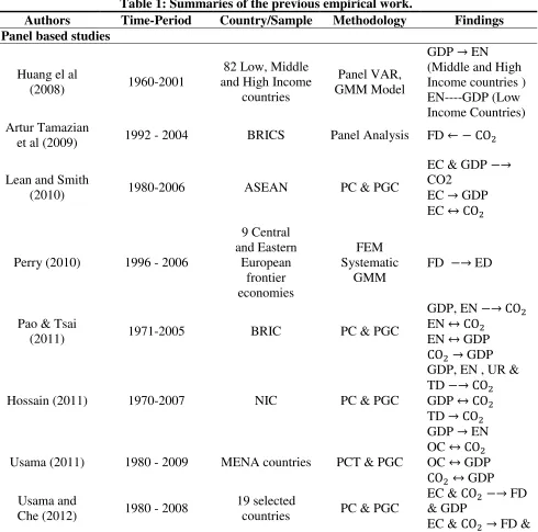
In sum up there is a relationship between energy consumption-Growth-Carbon emissions framework especially for the case of developing county like Pakistan. This study is the first empirical effort to evaluate the energy-growth-emissions nexus by incorporating trade openness and financial development indicators for the case of Pakistan where there are lack of comprehensive studies. Single county study will help in policy making decisions regarding environmental degradation. Summaries of the previous work is presented in Table 1.

Table 1: Summaries of the previous empirical work.

Authors Time-Period Country/Sample Methodology Findings

Panel based studies

Huang el al

(2008) 1960-2001

82 Low, Middle and High Income

countries

Panel VAR, GMM Model

GDP → EN

(Middle and High Income countries ) EN----GDP (Low Income Countries) Artur Tamazian

et al (2009) 1992 - 2004 BRICS Panel Analysis FD ← −CO2

Lean and Smith

(2010) 1980-2006 ASEAN PC & PGC

EC & GDP −→

CO2

EC → GDP

EC ↔CO₂

Perry (2010) 1996 - 2006

9 Central and Eastern

European frontier economies

FEM Systematic

GMM

FD −→ ED

Pao & Tsai

(2011) 1971-2005 BRIC PC & PGC

GDP, EN −→CO₂

EN ↔CO₂

EN ↔ GDP

CO2 → GDP

Hossain (2011) 1970-2007 NIC PC & PGC

GDP, EN , UR &

TD −→CO₂

GDP ↔CO₂

TD →CO₂

GDP → EN

Usama (2011) 1980 - 2009 MENA countries PCT & PGC

OC ↔CO₂

OC ↔ GDP

CO2 ↔ GDP

Usama and

Che (2012) 1980 - 2008

19 selected

countries PC & PGC

EC & CO₂ −→ FD

& GDP

GDP

Usama (2012) 1990 - 2009 12 Middle

Eastern countries

PC FMOLS

PGC

GDP ↔ FDI

FDI ↔ EN

EN ↔CO₂

CO2 ↔ TO

Usama and

Che (2012) 1980 - 2008

Sub Saharan

African countries PCT & PGC

EN ↔CO₂

GDP ↔ FD

FD ↔CO₂

Country Specific studies

Jumbe (2004) 1970-1999 Malawi JC & ECM GC EC ↔ GDP

NGDP → GDP

Wang et al

(2005) 1995-2007 China PC & PGC

GDP, EN −→CO₂

CO2 ↔ EN

EN ↔ GDP

GDP →CO₂

Gaolu and Chau

(2006) 1953 - 2002 China JC & GC EN → GDP

Jalil & Mahmud

(2009) 1975-2005 China

ARDL Model and Granger

Causality

GDP −→CO₂

Odhiambo

(2009) 1971-2006 Tanzania

ARDL Bounds

Tests EN → GDP

Abdul Jalil and, Mete Feridun

(2010)

1953 - 2006 China ARDL

FD ← −CO₂

GDP, EC & TO

−→CO2

Hatzigeorgou et

al (2011) 1977-2007 Greece JC & VECM GC

EN & GDP, −→

CO2

GDP →CO₂

EN ↔CO₂

Pao & Tsai

(2011) 1980-2007 Brazil JC & VECM GC

GDP, EN −→CO₂

CO2 ↔ EN

EN ↔ GDP

GDP ↔CO₂

Pao et al (2011) 1990 - 2007 Russia JC & VCEM GC GDP ↔ EN

Shahbaz and

Hooi (2012) 1971 - 2008 Tunisia

ARDL & VECM GC

FD ↔ EN

FD ↔ IND

EN ↔ IND

Jayanthakumaran

& Liu (2012) 1971-2007 China & India ARDL

GDP, TD & EN

−→CO2

Shahbaz et al

(2012) 1971-2009 Pakistan ARDL & VECM

GDP →CO₂

EN ↔CO₂

TO--- CO₂

Shahbaz et al

(2013) 1965 - 2008 South Africa

ARDL & VECM GC

GDP →CO₂

FD ← −CO₂

TO ← −CO₂

Shahbaz et al

(2013) 1971 - 2011 China ARDL & VECM

EC → GDP

EC ↔ FD

EC ↔ IT

FD ↔ IT

EC ↔ C

FD ↔ GDP

GDP ↔ IT

Ozturk and Ali

(2013) 1960 - 2007 Turkey ARDL & VECM FD → EC & GDP

Shahbaz (2013) 1975Q1–2011Q4 Indonesia ARDL

VECM

GDP & EC −→

CO2

FD & TO −→

GDP

EC ↔CO₂

GDP ↔ CO₂

FD →CO₂

Khalid et al

(2014) 1980 - 2013 Pakistan ARDL & VECM

GDP & TO −→

EC

GDP ↔ EC

Rashid Sbia et al

(2014) 1975Q1 - 2011Q4 UAE ARDL & VECM

FDI ↔ EN

FDI ↔CO₂

FDI ↔ GE

GDP ↔CO₂

GDP ↔ EN

EN ↔CO₂

Sakiru and

Shahbaz (2014) 1971-2012 Malaysia ARDL & VECM

NGC, FDI,

C & TO −→ GDP

NGC ↔ GDP

FDI ↔ GDP

NGC ↔ FDI

Note: ----, → & ↔ indicate no, unidirectional and bidirectional Granger causality, respectively. −→

& ← − represent positive and negative long run relationship. Abbreviations are as follow:

ARDL=Autoregressive Distributed Lags; BMI=Broad Money Investments; C=Capital;

CO2 =Carbon Emissions; EN=Energy Consumptions; ED=Energy Demand; FD=Financial

2. Econometric Methodology

2.1. Unit Root Testing

Various unit root test proposed in the literature e.g. ADF by Dickey and Fuller (1979),

DF-GLS by Elliot et al. (1996) and Ng–Perron by Ng and Perron (2001) have a potential

weakness that they are unable to take into account structural breaks, and hence may provide the biased results (Baum, 2004). These traditional unit root test normally encounter a type II error

i.e. failure to reject the null hypothesis of unit root when it’s false, when the time series haveone

or more structural breaks. The structural break unit root test developed by Clemente et al. (1998)

considers the presence of structural breaks and have therefore been applied in this paper.

Clemente et al. is appropriate when a time series has one or two structural breaks. The presence

of two structural breaks are tested based on the following null and alternative hypothesis:

𝐻0: 𝑦𝑡= 𝑦𝑡−1+ 𝛿1𝐷𝑇𝐵1𝑡+ 𝛿2𝐷𝑇𝐵2𝑡+ 𝑢𝑡 (1)

𝐻1: 𝑦𝑡= 𝑢 + 𝑑1𝐷𝑈1𝑡+ 𝑑2𝐷𝑇𝐵2𝑡+ 𝑒𝑡 (2)

Where, 𝐷𝑇𝐵_𝑖𝑡 is a pulse variable that takes the value 1 if t = 𝑇𝐵₁+1 (i =1, 2) and 0

otherwise. Further, 𝐷𝑈_𝑖𝑡 =1 if 𝑡 > 𝑇𝐵_𝑖 (i =1, 2) and 0 otherwise. TB and TB are the time periods

when the mean is being modified (Clemente et al., 1998). If the two breaks belong to the

innovational outlier, unit root hypothesis can be first estimated using the following model:

𝑦𝑡 = 𝜇 + 𝜌𝑦𝑡−1+ 𝛿1𝐷𝑇𝐵1𝑡+ 𝛿2𝐷𝑇𝐵2𝑡+ 𝑑1𝐷𝑈1𝑡+ 𝑑2𝐷𝑈2𝑡 + ∑ 𝑐𝑖Δ𝑦𝑡−𝑖 𝑁

𝑖=1

+ 𝑒𝑡 (3)

If the shifts in mean are considered as additive outliers, then the unit root null hypothesis can be tested through the following two-step procedure. First, the deterministic part of the variable is removed by estimating the following model:

𝑦𝑡 = 𝜇 + 𝑑1𝐷𝑈1𝑡+ 𝑑2𝐷𝑈2𝑡+ 𝑦̃𝑡 (4)

And, test of unit root is applied by searching for the minimal t-ratio for the r 51 hypothesis in the following model:

𝑦̃𝑡 = ∑ 𝜔1𝑖𝐷𝑇𝐵1𝑡−1 𝑁

𝑖=1

+ ∑ 𝜔2𝑖𝐷𝑇𝐵2𝑡−1 𝑁

𝑖=1

+ 𝜌𝑦̃𝑡−1+ ∑ 𝑐𝑖Δ𝑦̃𝑡−𝑖 𝑁

𝑖=1

+ 𝑒𝑡 (5)

2.2. ARDL Bound Testing for Cointegration

The Autoregressive Distributed Lag (ARDL) approach introduced by Pesaran and Smith

(1995) and modified by Pesaran et al. (2001) has several econometric advantages in comparison

to the traditional cointegration models. The approach can be applied regardless of the order of integration i.e. the variables may be stationary at levels or first difference. Traditional cointegration tests require all the variables to be integrated of order one. The ARDL bound

testing approach also assumes that all the variables are endogenous.1 Thus, we can apply ARDL

model to check cointegration among the variables of CO2 emission, economic growth, energy

consumption, financial development and trade openness. An ARDL representation of 𝐶𝑜₂

Omission (C), economic growth (G), energy consumption (EN), financial development (FD), and trade openness (OP) can be formulated as follows:

𝐶𝑡= 𝛼0+ 𝛼1𝐺𝑡+ 𝛼2𝐹𝐷𝑡+ 𝛼3𝐸𝑁𝑡+ 𝛼4𝑂𝑃𝑡+ 𝜇𝑡 (6)

The ARDL bound procedure to check the existence of cointegration is as under:

∆𝐶𝑡= 𝛼0+ 𝛼1𝐶𝑡−1+ 𝛼2𝐺𝑡−1+ 𝛼3𝐹𝐷𝑡−1+ 𝛼4𝐸𝑁𝑡−1+ 𝛼5𝑂𝑃𝑡−1+ ∑ 𝜃𝑖∆𝐶𝑡−𝑖 𝑝

𝑖=1

+ ∑ 𝜃𝑗∆𝐺𝑡−𝑗 𝑞

𝑗=1

+ ∑ 𝜃𝑘∆𝐹𝐷𝑡−𝑘 𝑟

𝐾=1

+ ∑ 𝜃𝑙∆𝐸𝑁𝑡−𝑙 𝑠

𝑙=1

+ ∑ 𝜃𝑙∆𝑂𝑃𝑡−𝑙 𝑇

𝑚=1

+ 𝜇𝑡 (7)

∆𝐺𝑡 = 𝛼0+ 𝛼1𝐶𝑡−1+ 𝛼2𝐺𝑡−1+ 𝛼3𝐹𝐷𝑡−1+ 𝛼4𝐸𝑁𝑡−1+ 𝛼5𝑂𝑃𝑡−1+ ∑ 𝜃𝑖∆𝐺𝑡−𝑖 𝑝

𝑖=1

+ ∑ 𝜃𝑗∆𝐶𝑡−𝑗 𝑞

𝑗=1

+ ∑ 𝜃𝑘∆𝐹𝐷𝑡−𝑘 𝑟

𝐾=1

+ ∑ 𝜃𝑙∆𝐸𝑁𝑡−𝑙 𝑠

𝑙=1

+ ∑ 𝜃𝑙∆𝑂𝑃𝑡−𝑙 𝑇

𝑚=1

+ 𝜇𝑡 (8)

∆𝐹𝐷𝑡 = 𝛼0+ 𝛼1𝐶𝑡−1+ 𝛼2𝐺𝑡−1+ 𝛼3𝐹𝐷𝑡−1+ 𝛼4𝐸𝑁𝑡−1+ 𝛼5𝑂𝑃𝑡−1+ ∑ 𝜃𝑖∆𝐹𝐷𝑡−𝑖 𝑝

𝑖=1

+ ∑ 𝜃𝑗∆𝐶𝑡−𝑗 𝑞

𝑗=1

+ ∑ 𝜃𝑘∆𝐺𝑡−𝑘 𝑟

𝐾=1

+ ∑ 𝜃𝑙∆𝐸𝑁𝑡−𝑙 𝑠

𝑙=1

+ ∑ 𝜃𝑙∆𝑂𝑃𝑡−𝑙 𝑇

𝑚=1

+ 𝜇𝑡 (9)

∆𝐸𝑁𝑡 = 𝛼0+ 𝛼1𝐶𝑡−1+ 𝛼2𝐺𝑡−1+ 𝛼3𝐹𝐷𝑡−1+ 𝛼4𝐸𝑁𝑡−1+ 𝛼5𝑂𝑃𝑡−1+ ∑ 𝜃𝑖∆𝐸𝑁𝑡−𝑖 𝑝

𝑖=1

+ ∑ 𝜃𝑗∆𝐶𝑡−𝑗 𝑞

𝑗=1

+ ∑ 𝜃𝑘∆𝐺𝑡−𝑘 𝑟

𝐾=1

+ ∑ 𝜃𝑙∆𝐹𝐷𝑡−𝑙 𝑠

𝑙=1

+ ∑ 𝜃𝑙∆𝑂𝑃𝑡−𝑙 𝑇

𝑚=1

+ 𝜇𝑡 (10)

∆𝑂𝑃𝑡 = 𝛼0+ 𝛼1𝐶𝑡−1+ 𝛼2𝐺𝑡−1+ 𝛼3𝐹𝐷𝑡−1+ 𝛼4𝐸𝑁𝑡−1+ 𝛼5𝑂𝑃𝑡−1+ ∑ 𝜃𝑖∆𝑂𝑃𝑡−𝑖 𝑝

𝑖=1

+ ∑ 𝜃𝑗∆𝐶𝑡−𝑗 𝑞

𝑗=1

+ ∑ 𝜃𝑘∆𝐺𝑡−𝑘 𝑟

𝐾=1

+ ∑ 𝜃𝑙∆𝐹𝐷𝑡−𝑙 𝑠

𝑙=1

+ ∑ 𝜃𝑙∆𝐸𝑁𝑡−𝑙 𝑇

𝑚=1

+ 𝜇𝑡 (11)

Cointegration procedure of Narayan (2005) has been adopted to verify the long run cointegration relationship between the variables; F or Wald-statistics are used for the bound testing. The test statistics is a joint significance test that test the null hypothesis of no cointegration against an alternative hypothesis that there is cointegration for equations (7) to 11) i.e.

𝐻0∶ 𝛼1 = 𝛼2 = 𝛼3= 𝛼4= 𝛼5= 0 (No cointegration)

𝐻1∶ 𝑎𝑡𝑙𝑒𝑎𝑠𝑡 𝑜𝑛𝑒 𝑜𝑓 𝑡ℎ𝑒 𝛼′𝑠 𝑖𝑠 𝑛𝑜𝑡 𝑒𝑞𝑢𝑎𝑙 𝑡𝑜 𝑍𝑒𝑟𝑜(Cointegration exists)

Narayan (2005) computed the critical values for a given significance level. The null

hypothesis i.e. no cointegration exists, can be rejected if the calculated F-statistic is higher than the upper critical bound. The critical values proposed by Narayan (2005) are considered appropriate when the sample size is small, therefore this paper used these values. After confirmation of the cointegration between the variables, next step is to estimate the long term coefficients. Several models have been proposed in the literature for long-run coefficient estimation i.e. OLS, Fully Modified OLS (FMOLS) and Dynamic OLS (DOLS). The relative strength and weakness of different OLS estimators have been examined by Chen et al. (1999). They suggest that later techniques can be promising to obtain the coefficients of cointegrated variables. The present study applies FMOLS and DOLS models to get the long run parameters for carbon emission, economic growth, energy consumption, financial development and trade openness.

2.3.1. The Fully Modified OLS (FMOLS) estimator

Due to biasness and inconsistency of the OLS estimates in a panel of cointegrated

variables, we have utilized the “group-mean” panel FMOLS developed by Pedroni [1999; 2001].

The coefficient estimates obtained through FMOLS model are consistent in relatively small sample and also control the possible endogeneity issue between the regressors. It also deal with the problem of serial correlation. Following FMOLS estimator for the i-th panel member is utilized in this study:

𝛽_𝑖∗_{= (𝑋}

𝑖′ 𝑋𝑖)−1(𝑋𝑖′𝑦𝑖∗− 𝑇𝛿), (12)

Where y* presents the transformed endogenous variable, T is the number of time periods and δ is a parameter for autocorrelation adjustment.

2.3.2. The Dynamic OLS (DOLS) estimator

To check the consistency of the FMOLS estimates, we have also analyzed the relationship between the variables by further applying DOLS technique. Similar to FMOLS, DOLS model also provide unbiased and estimators while correcting the potential endogeneity issue. DOLS achieves the previously mentioned estimates through parametric adjustment of error terms by adding both past and the future differenced I(1) values of the regressors. Following equation is used to obtain the Dynamic OLS estimator in present setting:

𝑌𝑖𝑡 = 𝛼𝑖 + 𝑋𝑖𝑡′ 𝛽 + ∑ 𝐶𝑖𝑗 𝑗=𝑞2

𝑗=−𝑞1

Δ𝑋𝑖𝑡+𝑗+ 𝑣𝑖𝑡, (13)

In the above mentioned equation X indicates all the independent variables i.e. G, FD, EN,

and OP. 𝐶_𝑖𝑗 indicates the coefficients for the lead or lag of first differenced independent

𝛽̂𝐷𝑂𝐿𝑆 = ∑( ∑ 𝑧𝑖𝑡𝑧𝑖𝑡′ 𝑇 𝑡=1 )−1 𝑁 𝑖=1

(∑ 𝑧𝑖𝑗 𝑇

𝑡=1

𝑦̂𝑖𝑡+), (14)

Where 𝑧_𝑖𝑡= [𝑋_𝑖𝑡- 𝑋̅_𝑖, ∆𝑋_{𝑖,𝑡−𝑞}, … … . ∆𝑋_{𝑖,𝑡+𝑞}] is vector of regressors, and 𝑦̂_𝑖𝑡+(𝑦̂_𝑖𝑡+= 𝑦_𝑖𝑡− 𝑦̅_𝑖) is the

carbon emmision variable.

2.2. Causality Analysis

The cointegration analysis can only reveal whether the causality is present or not; however, the direction of causality cannot be determined through ARDL procedure. If the variables are cointegrated then the direction of causality in bot short-run and long-run can be ascertained through the Granger causality approach. The Vector Error Correction (VECM) based Granger causality test applied is presented below:

∆𝐶𝑡= 𝛼01+ ∑ 𝛼11∆𝐶𝑡−𝑖 𝑛

𝑖=1

+ ∑ 𝛼22∆𝐺𝑡−𝑗 𝑝

𝑗=1

+ ∑ 𝛼33∆𝐹𝐷𝑡−𝑘 𝑞

𝑘=1

+ ∑ 𝛼44∆𝐸𝑁𝑡−𝑙 𝑟

𝑙=1

+ ∑ 𝛼55∆𝑂𝑃𝑡−𝑚 𝑠

𝑚=1

+ 𝜂1𝐸𝐶𝑀𝑡−1+ 𝜇1𝑡 (15)

∆𝐺𝑡 = 𝛽01+ ∑ 𝛽11∆𝐶𝑡−𝑖 𝑛

𝑖=1

+ ∑ 𝛽22∆𝐺𝑡−𝑗 𝑝

𝑗=1

+ ∑ 𝛽33∆𝐹𝐷𝑡−𝑘 𝑞

𝑘=1

+ ∑ 𝛽44∆𝐸𝑁𝑡−𝑙 𝑟

𝑙=1

+ ∑ 𝛽55∆𝑂𝑃𝑡−𝑚 𝑠

𝑚=1

+ 𝜂1𝐸𝐶𝑀𝑡−1+ 𝜇1𝑡 (16)

∆𝐹𝐷𝑡 = 𝛾01+ ∑ 𝛾11∆𝐶𝑡−𝑖 𝑛

𝑖=1

+ ∑ 𝛾22∆𝐺𝑡−𝑗 𝑝

𝑗=1

+ ∑ 𝛾33∆𝐹𝐷𝑡−𝑘 𝑞

𝑘=1

+ ∑ 𝛾44∆𝐸𝑁𝑡−𝑙 𝑟

𝑙=1

+ ∑ 𝛾55∆𝑂𝑃𝑡−𝑚 𝑠

𝑚=1

+ 𝜂1𝐸𝐶𝑀𝑡−1+ 𝜇1𝑡 (17)

∆𝐸𝑁𝑡 = 𝛿01+ ∑ 𝛿11∆𝐶𝑡−𝑖 𝑛

𝑖=1

+ ∑ 𝛿22∆𝐺𝑡−𝑗 𝑝

𝑗=1

+ ∑ 𝛿33∆𝐹𝐷𝑡−𝑘 𝑞

𝑘=1

+ ∑ 𝛿44∆𝐸𝑁𝑡−𝑙 𝑟

𝑙=1

+ ∑ 𝛿55∆𝑂𝑃𝑡−𝑚 𝑠

𝑚=1

+ 𝜂1𝐸𝐶𝑀𝑡−1+ 𝜇1𝑡 (18)

∆𝑂𝑃𝑡= 𝜃01+ ∑ 𝜃11∆𝐶𝑡−𝑖 𝑛

𝑖=1

+ ∑ 𝜃22∆𝐺𝑡−𝑗 𝑝

𝑗=1

+ ∑ 𝜃33∆𝐹𝐷𝑡−𝑘 𝑞

𝑘=1

+ ∑ 𝜃44∆𝐸𝑁𝑡−𝑙 𝑟

𝑙=1

+ ∑ 𝜃55∆𝑂𝑃𝑡−𝑚 𝑠

𝑚=1

+ 𝜂1𝐸𝐶𝑀𝑡−1+ 𝜇1𝑡 (19)

In eq. 15 to 19, ECTindicates the error correction term, 's present the error terms

assumed to be uncorrelated. The coefficient of the error correction term is denoted by



which indicates the speed of adjustment of ∆C_t, ∆G_t, ∆FD_t, ∆EN_t, and ∆OP_t, towards long run

equilibrium. In fact, the addition of EC term in the traditional Granger causality framework allows the emergences of causality and re-establishes the equilibrium relationship between the variables, in the event of a shock. Hence, by adding the ECT term, VECM can opens up new channels for Granger causality to emerge. Short term causality is captured through the estimated

coefficients of ∆C_t−1, ∆G_t−1, ∆FD_t−1, ∆EN_t−1, and ∆OP_t−1 . The positive and significant

3. Data and Findings

Annual time series data from 1973 to 2011 is used for the empirical work. Data on Carbon Emissions (Kilo Tons), Gross Domestic Product - GDP (Current $US) as a proxy for economic growth, Domestic Credit by Financial Sector (Current $US) as a proxy for financial development, Energy Consumption (Kilo tons of Oil equivalent) and trade openness (export plus

imports as a percentage of GDP) is taken from World Development Indicators (WDI) – 2014 by

the World Bank (WB). All variables are transformed in annual growth form.

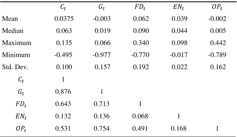
Table 2 provides descriptive statistics of the variables along with correlation matrix of the variables. Carbon emissions, financial development and energy consumption growth is positive in Pakistan over the sample period. Economic growth and trade openness have remained negative with a very low percentage growth. All the variables are positively correlated with each other. The result of simplistic correlation analysis is the start of study which calls for a further detailed framework to examine the potential relationship.

Table 2: Descriptive Statistics and Correlation Analysis

𝐶𝑡 𝐺𝑡 𝐹𝐷𝑡 𝐸𝑁𝑡 𝑂𝑃𝑡

Mean 0.0375 -0.003 0.062 0.039 -0.002

Median 0.063 0.019 0.090 0.044 0.005

Maximum 0.135 0.066 0.340 0.098 0.442

Minimum -0.495 -0.977 -0.770 -0.017 -0.789

Std. Dev. 0.100 0.157 0.192 0.022 0.162

𝐶𝑡 1

𝐺𝑡 0.876 1

𝐹𝐷𝑡 0.643 0.713 1

𝐸𝑁𝑡 0.132 0.136 0.068 1

𝑂𝑃𝑡 0.531 0.754 0.491 0.168 1

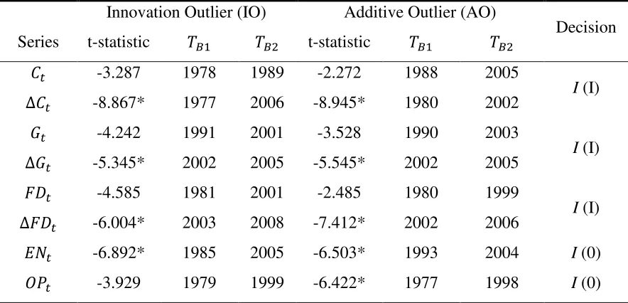
Tables 3 reports the results of Clemente–Montanes–Reyes detrended unit root test with

two structural breaks2. Results indicate presence of two structural breaks. Carbon emission,

economic growth and financial development are integrated of order one i.e. I(I) whereas energy

consumption and trade openness are stationary at level i.e. it is integrated of order one, I(0).

Since all variables do not have same level of integration, we will apply ARDL technique to find long run cointegration relationship among variables.

2_{The results report presence of two structural breaks in the time series data therefore, we have not reported the}

Table 3: Results of Clemente–Montanes–Reyes two structural break unit root test

Innovation Outlier (IO) Additive Outlier (AO)

Decision

Series t-statistic 𝑇_𝐵1 𝑇_𝐵2 t-statistic 𝑇_𝐵1 𝑇_𝐵2

𝐶𝑡 -3.287 1978 1989 -2.272 1988 2005

I (I)

∆𝐶𝑡 -8.867* 1977 2006 -8.945* 1980 2002

𝐺𝑡 -4.242 1991 2001 -3.528 1990 2003

I (I)

∆𝐺𝑡 -5.345* 2002 2005 -5.545* 2002 2005

𝐹𝐷𝑡 -4.585 1981 2001 -2.485 1980 1999

I (I)

∆𝐹𝐷𝑡 -6.004* 2003 2008 -7.412* 2002 2006

𝐸𝑁𝑡 -6.892* 1985 2005 -6.503* 1993 2004 I (0)

𝑂𝑃𝑡 -3.929 1979 1999 -6.422* 1977 1998 I (0)

Note: * indicates significance at 5% level.

To ascertain the existence of a long run cointegrating relationship among carbon emission, economic growth, financial development, energy consumption and trade openness, the bounds testing approach is applied. Moreover, the selection of lag length should be performed carefully because an inappropriate lag length may lead to biased results and is not acceptable for policy analysis. Therefore, to ensure that the lag length was selected appropriately. Results of Akaike information criteria (AIC), Schwartz Bayesian criteria (SBC) and Hannan-Quinn information criterion (HQ) are reported in Table 4. Based on Akaike information criterion (AIC), Schwarz information criterion (SC) and Hannan-Quinn information criterion (HQ), optimal lag length 1 is selected for causality analysis (Table 4).

Table 4: Lag Order Selection

Lag LogL LR FPE AIC SC HQ

0 322.212 NA 1.53e-14 -17.622 -17.402 -17.546

1 351.712 49.168* 1.21e-14* -17.872* -16.553* -17.412*

2 376.430 34.329 1.34e-14 -17.857 -15.437 -17.012

3 406.526 33.440 1.27e-14 -18.140 -14.621 -16.912

Note: * indicates lag order selected by the criterion; LR=sequential modified LR test statistic (each test at 5% level); FPE-=Final prediction error; AIC=Akaike information criterion; SC=Schwarz information criterion; HQ=Hannan-Quinn information criterion

After determining the optimal lag length, we have applied F-statistics to check the

is a long run cointegrating relationship between the selected variables. F statistics value are 20.887, 7.262 and 8.426 when carbon emission, energy consumption and trade openness are considered as dependent variables (Eq. 7, 10 & 11) respectively. The F statistics are significant at 1% level because it is higher than the upper critical bounds of Narayan (2005). The results for economic growth and financial development (Eq. 8 & 9) are inconclusive.

Table 5: Bound Test for Cointegration (1973 – 2011)

Critical values (lower and upper bound) of the F statistics: intercept and no trend

Tabulated F Statistics (T=40, K=4)

I(0) I(I)

90% level 2.660 3.838

95% level 3.202 4.544

99% level 4.428 6.250

Estimated Models Calculated F statistics

𝐸𝑞. 2; 𝐶𝑡= 𝑓(𝐺𝑡, 𝐹𝐷𝑡, 𝐸𝑁𝑡, 𝑂𝑃𝑡) 20.887*

𝐸𝑞. 3; 𝐺𝑡= 𝑓(𝐶𝑡, 𝐹𝐷𝑡, 𝐸𝑁𝑡, 𝑂𝑃𝑡) 6.154

𝐸𝑞. 4; 𝐹𝐷𝑡 = 𝑓(𝐶𝑡, 𝐺𝑡, 𝐸𝑁𝑡, 𝑂𝑃𝑡) 3.557

𝐸𝑞. 5; 𝐸𝑁𝑡= 𝑓(𝐶𝑡, 𝐺𝑡, 𝐹𝐷𝑡, 𝑂𝑃𝑡) 7.262*

𝐸𝑞. 6; 𝑂𝑃𝑡 = 𝑓(𝐶𝑡, 𝐺𝑡, 𝐹𝐷𝑡, 𝐸𝑁𝑡) 8.426*

Note: * indicates that F-statistic falls above the 1% upper bound. Reported critical values are from Narayan (2005).

The ARDL bound testing procedure to ascertain a long-run relationship between carbon emission, economic growth, energy consumption, financial development and trade openness in Pakistan show that there are three cointegration vectors. The cointegration exits as the calculated F statistics falls above the upper critical values provided by Narayan (2005). The authenticity of the cointegration equation is made by testing the assumption of Classical Linear Regression Model (CLRM). Results presented below (Table 6) show that different diagnostic tests reject the null hypothesis at 10% level of significance. The tests result in combination confirm that there is no problem of non-normality, serial correlation and conditional heteroskedasticity in the long-run ARDL bound testing equations. The model specification is tested by applying Ramsey RESET test which indicates that models are correctly specified.

Table 6: The Results of Diagnostic Tests

Equation 2 3 4 5 6

Diagnostic Tests

R Square 0.863 0.575 0.654 0.610 0.659

F-statistics 18.940

(0.000)

4.059 (0.002)

3.208 (0.000)

4.704 (0.000)

5.815 (0.000)

JB Normality Test 0.693

(0.706)

0.729 (0.694)

0.936 (0.625)

4.307 (0.116)

0.457 (0.795)

Breusch–Godfrey LM test 0.225

(0.720)

0.614 (0.420)

0.354 (0.540)

0.183 (0.765)

1.448 (0.146)

(0.226) (0.321) (0.143) (0.355) (0.135)

Ramsey RESET 2.804

(0.106)

0.102 (0.751)

1.839 (0.189)

0.790 (0.382)

7.455 (0.011) Note: * , ** and *** indicate that values are significance at 1%, 5% and 10% levels of significance respectively.

The stability of the long and short run parameters in the ARDL bound testing equations is further examined by applying cumulative sum (CUSUM) and cumulative sum of squares (CUSUMsq) tests (Pesaran and Shin, 1999). Figs. 5 and 6 indicate the graphs of CUSUM and CUSUMsqare, respectively. Both the graphs indicate the CUSUM and CUSUMsqare values are between the critical boundaries at 5% level of significance. As the calculated values shown in the graph are between the critical boundaries, the long and short run parameters which have effect on carbon emission in Pakistan, are assumed to stable. These stability tests further confirm that there are no structural breaks and hence no impact on the ARDL bound testing equations. Based on above mentioned diagnostic and stability tests, we can conclude that the ARDL model seems to be steady and appropriately specified.

-15 -10 -5 0 5 10 15

88 90 92 94 96 98 00 02 04 06 08 10

CUSUM 5% Significance

Fig.1. Graph of Cumulative Sum of Recursive Residuals

-0.4 -0.2 0.0 0.2 0.4 0.6 0.8 1.0 1.2 1.4

88 90 92 94 96 98 00 02 04 06 08 10

CUSUM of Squares 5% Significance

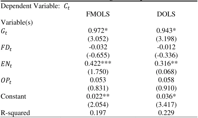
Tables 7 display the results of FMOLS and DOLS using carbon emission as the dependent variable. The economic growth and energy consumption coefficients are positive and significant in Pakistan. The positive (+) coefficients suggests that increase in economic growth and energy consumption leads to increase in carbon emission in Pakistan. One percent increase in economic growth and energy consumption lead to 0.97% and 0.42% increase in carbon emission, respectively. The coefficients of financial development and trade openness are insignificant and thus do not impact the carbon emissions in the long run. Results of both FMOLS and DOLS are consistent and almost similar in magnitude.

Table 7: Result of Cointegration Equations

Dependent Variable: 𝐶_𝑡

FMOLS DOLS

Variable(s)

𝐺𝑡 0.972*

(3.052)

0.943* (3.198)

𝐹𝐷𝑡 -0.032

(-0.655)

-0.012 (-0.336)

𝐸𝑁𝑡 0.422***

(1.750)

0.316** (0.068)

𝑂𝑃𝑡 0.053

(0.831)

0.058 (0.910)

Constant 0.022**

(2.054)

0.036* (3.417)

R-squared 0.197 0.229

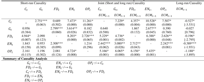
VECM based Granger Causality approach is applied to examine the direction of causality for carbon emission, economic growth, financial development, energy consumption and trade openness. Zeller (1998) suggest that causality can be interpreted in purely probability sense, not in deterministic terms. Table 8 reports the results of both short and long run causality estimates. The t statists is used to determine the significance of lagged ECT and hence proves the long run relationship. The significance of Wald test on sum of lags of independent variables in Eq. (15) to Eq. (19) is used to determine the existence of short term causality relation. This interpretation is

similar to Masih and Masih (1996). Carbon emissions are impacted by economic growth, energy

Table 8: Vector Error Correction Model: Causality Analysis

Short-run Causality Joint (Short and long run) Causality Long-run Causality 𝐶𝑡 𝐺𝑡 𝐹𝐷𝑡 𝐸𝑁𝑡 𝑂𝑃𝑡 𝐶𝑡,

𝐸𝐶𝑀𝑡−1

𝐺𝑡,

𝐸𝐶𝑀𝑡−1

𝐹𝐷𝑡,

𝐸𝐶𝑀𝑡−1

𝐸𝑁𝑡,

𝐸𝐶𝑀𝑡−1

𝑂𝑃𝑡,

𝐸𝐶𝑀𝑡−1

𝐸𝐶𝑀𝑡−1

𝐶𝑡 - 2.751***

(0.063) 0.689 (0.502) 7.473* (0.000) 11.261* (0.000)

- 7.229* (0.000) 4.357* (0.004) 10.528* (0.000) 7.507* (0.000) -0.527* [-3.531] 𝐺𝑡 0.956

(0.384)

- 2.799*** (0.060) 3.614** (0.026) 0.182 (0.832) 0.640 (0.588)

- 1.867 (0.132) 2.677** (0.045) 0.390 (0.760) -0.027 [0.796] 𝐹𝐷𝑡 4.944*

(0.007)

2.090 (0.123)

- 8.203* (0.000) 2.726*** (0.065) 5.229* (0.001) 4.736* (0.002)

- 6.388* (0.000)

2.626** (0.048)

-0.196* [-2.795] 𝐸𝑁𝑡 1.843

(0.158)

0.953 (0.385)

2.308*** (0.099)

- 1.214 (0.296) 2.442*** (0.062) 3.080** (0.026) 2.712** (0.043)

- 2.242*** (0.081)

-0.389*** (-1.931) 𝑂𝑃𝑡 2.161

(0.115) 1.196 (0.302) 2.081 (0.124) 4.724* (0.008)

- 5.166* (0.001) 6.065* (0.000) 6.156* (0.000) 5.435* (0.001)

- -1.188* (-3.895)

Summary of Causality Analysis

𝐺𝑡−∕→𝐶𝑡 𝐸𝑁𝑡−∕→𝐶𝑡 𝑂𝑃𝑡−∕→𝐶𝑡

𝐹𝐷𝑡−∕→𝐺𝑡 𝐸𝑁𝑡−∕→𝐺𝑡

𝐶𝑡−∕→𝐹𝐷𝑡 𝐸𝑁𝑡−∕→𝐹𝐷𝑡 𝑂𝑃𝑡−∕→𝐹𝐷𝑡

𝐹𝐷𝑡−∕→𝐸𝑁𝑡

𝐸𝑁𝑡−∕→𝑂𝑃𝑡

Note: * , ** and *** indicate that values are significance at 1%, 5% and 10% levels of significance respectively. P-values (F-statistics) are in (). Student

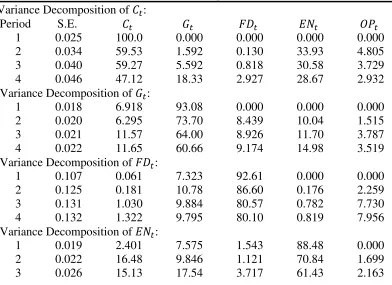
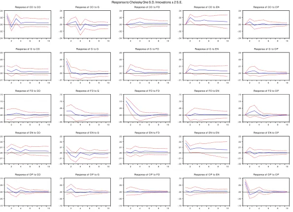
Wolde-Rufael (2009) argues that Granger causality is unable to determine the cause and effect relationship between the variables beyond the observed time period. Thus the reliability of Granger causality to capture the feedback amongst the variables is significantly decreased. Wolde-Rufael (2009) highlights the importance of Variance decomposition analysis (VDA) to establish the direction as well as strength of causality ahead of time. It also helps to examine the feedback effect from one variable to another. This paper applies both VDA and Impulse Response Function (IRF) for such analysis as both techniques are considered alternates to each other. Both the preceding methods help to capture the error variance of dependent variable(s) in response to shock or change occurring in independent variable over future time periods. Results reported in Table 9 indicate the VDA values for all five equations where carbon emission, economic growth, financial development, energy consumption and trade openness as dependent variables are reported from top to down, respectively. 47.12% of carbon emissions are impacted by own innovative shocks in a four year time period. Energy consumption and economic growth explains 28.67% and 18.33% of carbon emissions through their innovative shocks. 60.66% of growth variation is explained through its own innovations. 14.98%, 11.65 and 9.17% of variation in growth is through shocks in energy consumption, carbon emissions and financial development, respectively. 80.10% variation in financial development is explained by its own innovations. Economic growth explains 9.79% variations in financial development through its innovative shocks and trade openness explains 7.95%. Energy consumption and trade openness are majorly impacted by the innovation in economic growth and carbon emissions. The findings of VDA confirm the findings of VECM granger causality analysis. Similar findings are also evident through Impulse response function (figure 1). Finally, there are three cointegration vectors between carbon emissions, economic growth, energy consumption, financial development and trade openness in case of Pakistan using annual data from 1973 to 2011.

Table 9: Variance Decomposition Analysis

Variance Decomposition of 𝐶_𝑡:

Period S.E. 𝐶_𝑡 𝐺_𝑡 𝐹𝐷_𝑡 𝐸𝑁_𝑡 𝑂𝑃_𝑡

1 0.025 100.0 0.000 0.000 0.000 0.000

2 0.034 59.53 1.592 0.130 33.93 4.805

3 0.040 59.27 5.592 0.818 30.58 3.729

4 0.046 47.12 18.33 2.927 28.67 2.932

Variance Decomposition of 𝐺_𝑡:

1 0.018 6.918 93.08 0.000 0.000 0.000

2 0.020 6.295 73.70 8.439 10.04 1.515

3 0.021 11.57 64.00 8.926 11.70 3.787

4 0.022 11.65 60.66 9.174 14.98 3.519

Variance Decomposition of 𝐹𝐷_𝑡:

1 0.107 0.061 7.323 92.61 0.000 0.000

2 0.125 0.181 10.78 86.60 0.176 2.259

3 0.131 1.030 9.884 80.57 0.782 7.730

4 0.132 1.322 9.795 80.10 0.819 7.956

Variance Decomposition of 𝐸𝑁_𝑡:

1 0.019 2.401 7.575 1.543 88.48 0.000

2 0.022 16.48 9.846 1.121 70.84 1.699

4 0.027 13.88 15.67 3.523 64.97 1.939

Variance Decomposition of 𝑂𝑃_𝑡:

1 0.080 14.36 0.566 0.032 0.997 84.04

2 0.086 12.81 7.989 0.735 0.915 77.54

3 0.088 13.50 8.016 0.824 2.324 75.33

Figure 3: Impulse Response Function analysis -.04 -.02 .00 .02 .04

2 4 6 8 10

Response of CO to CO

-.04 -.02 .00 .02 .04

2 4 6 8 10

Response of CO to G

-.04 -.02 .00 .02 .04

2 4 6 8 10

Response of CO to F D

-.04 -.02 .00 .02 .04

2 4 6 8 10

Response of CO to EN

-.04 -.02 .00 .02 .04

2 4 6 8 10

Response of CO to O P

-.01 .00 .01 .02 .03

2 4 6 8 10

Response of G to CO

-.01 .00 .01 .02 .03

2 4 6 8 10

Response of G to G

-.01 .00 .01 .02 .03

2 4 6 8 10

Response of G to F D

-.01 .00 .01 .02 .03

2 4 6 8 10

Response of G to EN

-.01 .00 .01 .02 .03

2 4 6 8 10

Response of G to O P

-.05 .00 .05 .10 .15

2 4 6 8 10

Response of F D to CO

-.05 .00 .05 .10 .15

2 4 6 8 10

Response of F D to G

-.05 .00 .05 .10 .15

2 4 6 8 10

Response of F D to F D

-.05 .00 .05 .10 .15

2 4 6 8 10

Response of F D to EN

-.05 .00 .05 .10 .15

2 4 6 8 10

Response of F D to O P

-.02 -.01 .00 .01 .02 .03

2 4 6 8 10

Response of EN to CO

-.02 -.01 .00 .01 .02 .03

2 4 6 8 10

Response of EN to G

-.02 -.01 .00 .01 .02 .03

2 4 6 8 10

Response of EN to F D

-.02 -.01 .00 .01 .02 .03

2 4 6 8 10

Response of EN to EN

-.02 -.01 .00 .01 .02 .03

2 4 6 8 10

Response of EN to O P

-.10 -.05 .00 .05 .10

2 4 6 8 10

Response of O P to CO

-.10 -.05 .00 .05 .10

2 4 6 8 10

Response of O P to G

-.10 -.05 .00 .05 .10

2 4 6 8 10

Response of O P to F D

-.10 -.05 .00 .05 .10

2 4 6 8 10

Response of O P to EN

-.10 -.05 .00 .05 .10

2 4 6 8 10

Different ordering of the independent variables are considered to have significant implications on the results of variance decompositions and impulse response. Change in the order may change the results of both these tests. In the present empirical setting, five variables

can have 120 (5!) different ordering pairs. The robustness of the results while changing the order

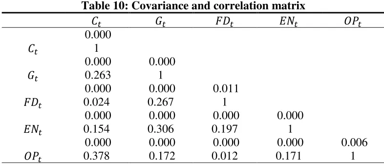
of variables for 120 times is almost next to impossible and also cumbersome. Masih and Masih (1996) proposed an alternate to solve this puzzle. They suggest that the covariance matrix of the error term obtained through reduced form VAR can be examined to ensure the consistency of VDA and IRF results. If the covariance matrix of the errors are close to diagonal then we can conclude that different orders of variables will not influence the structural inference. The covariance matrix of the residual is reported in Table 10. Results indicate that covariance matrix

is almost diagonal and hence it can be concluded variables’ orderings have no impact on the IRF

and VDA errors. An alternative method to ensure this conclusion, is to examine the statistical significance of correlation between the error terms. If the correlation between the errors is high and significance (based on traditional t statistics) then it is can be inferred that different identifying restrictions have a potential impact on the results. If no significance relationship between the errors exits then identification restriction cannot influence the results of VDA and IRF. The lower values in the table 10 reports the correlation between the errors. Results indicate

that residuals’ correlations is weak and statistically insignificant. Both diagnostic tests confirm that results of VDA and IRF are not sensitive to the change in identifying restrictions.

Table 10: Covariance and correlation matrix

𝐶𝑡 𝐺𝑡 𝐹𝐷𝑡 𝐸𝑁𝑡 𝑂𝑃𝑡

𝐶𝑡

0.000 1

𝐺𝑡

0.000 0.263

0.000 1

𝐹𝐷𝑡

0.000 0.024

0.000 0.267

0.011 1

𝐸𝑁𝑡

0.000 0.154

0.000 0.306

0.000 0.197

0.000 1

𝑂𝑃𝑡

0.000 0.378

0.000 0.172

0.000 0.012

0.000 0.171

0.006 1 Note: The upper values are of covariance and lower values show correlation.

4. CONCLUSION

Short run relationship is determined through Vector Error Correction (VEC) based Granger causality, Variance Decomposition Analysis (VDA) and Impulse Response Function (IRF). The presence of long run cointegration between the variables is confirmed. We find that carbon emissions increases with the increase in economic growth and energy consumption in long run. The results show that there is a unidirectional causality running from growth, energy consumption and trade openness to carbon emission. Financial development and energy consumption cause economic growth. Carbon emissions and trade openness cause financial development. Trade openness also Granger causes energy consumption. There is a bi-directional causality between financial development and energy consumption in Pakistan. Hence, the efforts to overcome energy crises and foster the economic growth require considerable attention to the carbon emissions; the best policy is to improve the situation through alternate energy resources

i.e. coal, LPG and LNG. The formulation as well as enforcement of environmental protection

laws is also required. Efficient and conservative use of scarce energy resources can spur the economic growth while limiting the degradation of environment.

REFERENCES

Ahmed, K., Shahbaz, M., Qasim, A., & Long, W. (2015). The linkages between deforestation,

energy and growth for environmental degradation in Pakistan. Ecological Indicators, 49, 95-103.

Al-Mulali, U. (2011). Oil consumption, CO₂ emission and economic growth in MENA

countries. Energy, 36(10), 6165-6171.

Al-mulali, U. (2012). Factors affecting CO₂ emission in the Middle East: A panel data

analysis. Energy, 44(1), 564-569.

Al-Mulali, U., & Binti Che Sab, C. N. (2012). The impact of energy consumption and CO₂

emission on the economic growth and financial development in the Sub Saharan African

countries. Energy, 39(1), 180-186.

Antweiler, W., Copeland, B. R., & Taylor, M. S. (1998). Is free trade good for the

environment? (No. w6707). National bureau of economic research.

Bacon, Robert W.; Bhattacharya, Soma. 2007. Growth and 𝐶𝑂₂ emissions: how do different

countries fare?. Environment working paper series; no. 113. Washington, DC: World Bank. Kuznets, S. (1955). Economic growth and income inequality. The American economic review,

1-28.

http://documents.worldbank.org/curated/en/2007/11/8838217/growth-co2-emissions-different-countries-fare.

Baum, C.F., (2004). A review of Stata 8.1 and its time series capabilities. International Journal

of Forecasting, 20(1), 151–161.

Clemente, J., Montanes, A., Reyes, M., (1998). Testing for a unit root in variables with a double

change in the mean. Economics Letters, 59(2), 175–182.

Cole, C. V., Duxbury, J., Freney, J., Heinemeyer, O., Minami, K., Mosier, A., & Zhao, Q.

(1997). Global estimates of potential mitigation of greenhouse gas emissions by

agriculture. Nutrient Cycling in Agroecosystems, 49(1-3), 221-228.

Dickey, D., Fuller, W.A., (1979). Distribution of the estimates for autoregressive time series with

unit root. Journal of the American Statistical Association, 74(366), 427–431.

Elliot, G., Rothenberg, T.J., Stock, J.H., (1996). Efficient tests for an autoregressive unit root.

Hatzigeorgiou, E., Polatidis, H., & Haralambopoulos, D. (2011). CO₂ emissions, GDP and

energy intensity: A multivariate cointegration and causality analysis for Greece, 1977–

2007. Applied Energy, 88(4), 1377-1385.

Heckscher E. The effect of foreign trade on the distribution of income. Ekonimisk Tidskriff

1919:497-512 and Ohlin B. Interregional and international trade. Harvard, MA: Cambridge University Press; 1933.

Hossain, S. (2011). Panel estimation for CO₂ emissions, energy consumption, economic growth,

trade openness and urbanization of newly industrialized countries. Energy Policy, 39(11),

6991-6999.

Huang, B. N., Hwang, M. J., & Yang, C. W. (2008). Causal relationship between energy

consumption and GDP growth revisited: a dynamic panel data approach. Ecological

economics, 67(1), 41-54.

Jalil, A., & Feridun, M. (2011). The impact of growth, energy and financial development on the

environment in China: A cointegration analysis. Energy Economics, 33(2), 284-291.

Jalil, A., & Mahmud, S. F. (2009). Environment Kuznets curve for co2 emissions: A

cointegration analysis for China. Energy Policy, 37(12), 5167-5172.

Jayanthakumaran, K., Verma, R., & Liu, Y. (2012). CO₂ emissions, energy consumption, trade

and income: A comparative analysis of China and India. Energy Policy, 42, 450-460.

Jumbe, C. B. (2004). Cointegration and causality between electricity consumption and GDP:

empirical evidence from Malawi. Energy economics, 26(1), 61-68.

Karanfil, F. (2009). How many times again will we examine the energy-income nexus using a

limited range of traditional econometric tools?. Energy Policy, 37(4), 1191-1194.

Lean, H. H., & Smyth, R. (2010). CO₂ emissions, electricity consumption and output in

ASEAN. Applied Energy, 87(6), 1858-1864.

Masih, A. M., & Masih, R. (1996). Energy consumption, real income and temporal causality: results from a multi-country study based on cointegration and error-correction modelling

techniques. Energy Economics, 18(3), 165-183.

Muhammad, S., Qazi Muhammad Adnan, H., & Aviral Kumar, T. (2013). Economic Growth,

Energy Consumption, Financial Development, International Trade and CO₂ Emissions, in

Indonesia. Renewable and Sustainable Energy Reviews, 25, 109-121.

Muhammad, S., Tiwari, A., & Muhammad, N. (2011). The effects of financial development, economic growth, coal consumption and trade openness on environment performance in South

Africa.Energy Policy, 61, 1452-1459.

Narayan, P.K., (2005). The saving and investment nexus for China: evidence from cointegration

tests. Applied Economics, 37(17), 1979–1990.

Ng, S., Perron, P., (2001). Lag length selection and the construction of unit root test with good

size and power. Econometrica, 69(6), 1519–1554.

Odhiambo, N. M. (2009). Energy consumption and economic growth nexus in Tanzania: an

ARDL bounds testing approach. Energy Policy, 37(2), 617-622.

Ozturk, I., & Acaravci, A. (2013). The long-run and causal analysis of energy, growth, openness

and financial development on carbon emissions in Turkey. Energy Economics, 36, 262-267.

Pao, H. T., & Tsai, C. M. (2011). Modeling and forecasting the CO₂ emissions, energy

consumption, and economic growth in Brazil. Energy, 36(5), 2450-2458.

Pao, H. T., & Tsai, C. M. (2011). Multivariate Granger causality between CO₂ emissions, energy

a panel of BRIC (Brazil, Russian Federation, India, and China) countries. Energy, 36(1), 685-693.

Pao, H. T., Yu, H. C., & Yang, Y. H. (2011). Modeling the CO₂ emissions, energy use, and

economic growth in Russia. Energy, 36(8), 5094-5100.

Pedroni, P. (2001). Fully modified OLS for heterogeneous cointegrated panels. Advances in

econometrics, 15, 93-130.

Pedroni, P., (1999). Critical values for cointegration tests in heterogeneous panels with multiple

regressors. Oxford Bulletin of Economics and Statistics, 61, 653–670.

Pesaran, M. H., & Smith, R. (1995). Estimating long-run relationships from dynamic

heterogeneous panels. Journal of econometrics, 68(1), 79-113.

Pesaran, M.H., Shin, Y., Smith, R.J., (2001). Bounds testing approaches to the analysis of level

relationships. Journal of Applied Econometrics, 16(3), 289–326.

Sadorsky, P. (2010). The impact of financial development on energy consumption in emerging

economies. Energy Policy, 38(5), 2528-2535.

Sbia, R., Shahbaz, M., & Hamdi, H. (2014). A contribution of foreign direct investment, clean energy, trade openness, carbon emissions and economic growth to energy demand in

UAE. Economic Modelling, 36, 191-197.

Shahbaz, M., & Lean, H. H. (2012). Does financial development increase energy consumption?

The role of industrialization and urbanization in Tunisia. Energy Policy, 40, 473-479.

Shahbaz, M., Khan, S., & Tahir, M. I. (2013). The dynamic links between energy consumption, economic growth, financial development and trade in China: fresh evidence from multivariate

framework analysis. Energy Economics, 40, 8-21.

Shahbaz, M., Lean, H. H., & Shabbir, M. S. (2012). Environmental Kuznets curve hypothesis in

Pakistan: cointegration and Granger causality. Renewable and Sustainable Energy

Reviews, 16(5), 2947-2953.

Solarin, S. A., & Shahbaz, M. (2015). Natural gas consumption and economic growth: The role

of foreign direct investment, capital formation and trade openness in Malaysia. Renewable and

Sustainable Energy Reviews, 42, 835-845.

Wang, C., Chen, J., & Zou, J. (2005). Decomposition of energy-related CO₂ emission in China:

1957–2000. Energy, 30(1), 73-83.

Wolde-Rufael, Y., (2009).The defence spending-external debt nexus in Ethiopia. Defence and

Peace Economics, 20(5), 423–436.

Zellner, A. (1988). Causality and causal laws in economics. Journal of Econometrics, 39, 7-21.

Zou, G., & Chau, K. W. (2006). Short-and long-run effects between oil consumption and