Simplified Coarse Grained Dynamic Model for Real Gases

http://www.scirp.org/journal/ojpc ISSN Online: 2162-1977

ISSN Print: 2162-1969

Simplified Coarse-Grained Dynamic

Model for Real Gases

Panagis G. Papadopoulos

, Christopher G. Koutitas

, Yannis N. Dimitropoulos

, Elias C. Aifantis

1_{Department of Civil Engineering, Aristotle University of Thessaloniki, Thessaloniki, Greece} 2_{Department of Chemistry, University of Ioannina, Ioannina, Greece}

Abstract

A simplified model is proposed for an easy understanding of the coarse- grained technique and for achieving a first approximation to the behavior of gases. A mole of a gas substance, within a cubic container, is represented by six particles symmetrically moving. The impacts of particles on container walls, the inter-particle collisions, as well as the volume of particles and the inter-particle attractive forces, obeying a Lennard-Jones curve, are taken into account. Thanks to the symmetry, the problem is reduced to the nonlinear dynamic analysis of a SDOF oscillator, which is numerically solved by a step- by-step time integration algorithm. Five applications of proposed model, on Carbon Dioxide, are presented: 1) Ideal gas in STP conditions. 2) Real gas in STP conditions. 3) Condensation for small molar volume. 4) Critical point. 5) Iso-kinetic energy curves and iso-therms in the critical point region. Results of the proposed model are compared with test data and results of the Van der Waals model for real gases.

Keywords

Real Gases, Coarse-Grained Molecular Dynamics, Particles Volume, Inter-Particle Attractive Forces, Lennard-Jones Curve, Step-by-Step Time Integration Algorithm, Condensation, Critical Point,

Iso-Kinetic Energy Curves, Iso-Therms, Van der Waals Model

1. Introduction

Recently, in Computational Chemistry, the coarse-grained molecular dynamics technique is often used, by which millions of molecules are represented by a few hundred particles [1]-[13]. For example, if a mole of a gas substance is simulated by a thousand particles, by use of Avogadro number, it is noticed that every par-ticle represents about 6 × 1020 _{molecules. By this technique, the computational}

How to cite this paper: Papadopoulos, P.G., Koutitas, C.G., Dimitropoulos, Y.N. and Aifantis, E.C. (2017) Simplified Coarse- Grained Dynamic Model for Real Gases. Open Journal of Physical Chemistry, 7, 50-71.

https://doi.org/10.4236/ojpc.2017.72005

Received: April 13, 2017 Accepted: May 13, 2017 Published: May 16, 2017

Copyright © 2017 by authors and Scientific Research Publishing Inc. This work is licensed under the Creative Commons Attribution International License (CC BY 4.0).

handling of chemical problems becomes possible and usually a satisfactory ap-proximation to observed behavior is achieved.

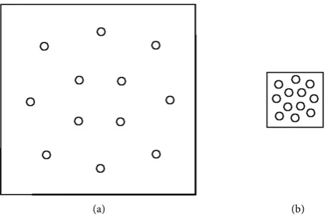
If we consider an amount of a gas substance, represented by a few particles, first in a large container (Figure 1(a)) and then in a small container (Figure 1(b)), the following two observations can be made [14]:

1.In the large container of Figure 1(a), the volume of particles is not significant, compared with the volume of the container. On the contrary, in the small container of Figure 1(b), the volume of particles is significant.

2.In the large container of Figure 1(a), the mean distance between a couple of particles is large, so, as well known from Physical Chemistry [14] and de-scribed by Lennard-Jones curve [15], the inter-particle attractive forces result small up to negligible. On the contrary, in the small container, the mean dis-tance, between a couple of particles, is small, so the inter-particle attractive forces exhibit significant values.

For the above two reasons, for a quite large molar volume, as in Figure 1(a), the volumes of particles and the inter-particle attractive forces can be ignored. So, the amount of gas substance under consideration obeys the ideal gas laws.

On the contrary, for a small molar volume, as in Figure 1(b), the particles volumes and the inter-particle attractive forces must be taken into account. That is, we have a real gas, which significantly deviates from the behavior of ideal gases.

J. D. van der Waals [16], by taking into account the molecular volumes and the inter-molecular attractive forces, developed a semi-rational, semi-empirical model, which is simple and exhibits a satisfactory approximation to the observed behavior of real gases.

The kinetic behavior of gases, ideal and real ones, is often described by the Maxwell-Boltzmann stochastic model [17]. The stochastic models are accurate but complicated. On the other hand, they obey some required symmetries. And it is recognized [18] [19] that, alternatively to a stochastic model, a symmetric deterministic model can be used, which is much simpler, but usually exhibits sa-tisfactory approximation to test data.

(a) (b)

Also, a very coarse-grained model can be used, that is consisting of very few, very large particles. This is similar to the concept of fundamental vibration mode of structural dynamics. Where there exist a lot of high vibration modes (with small periods and usually small amplitudes, too), which are of negligible interest, but complicate the computation and require a very small time steplength. Whe-reas, the fundamental vibration mode is the simplest mode and, at the same time, the most representative of the dynamic behavior of the structure.

In the present work, such a symmetric deterministic model is proposed for real gases, which is very coarse-grained, that is, it consists of very few - very large particles, and is compared to corresponding test data [14] [20], as well as to re-sults of the Van der Waals model [14] [16] for real gases.

In the recent literature on the coarse-grained technique [1]-[13], advanced models are proposed, for the accurate description of the behavior of real mate-rials, which can be used in the Design. Whereas, the proposed here simplified model, aims to an easy understanding, of the coarse-grained technique, by re-searchers of other than Chemistry fields and to a first approximation to the be-havior of gases.

2. Proposed Model

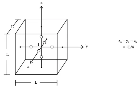
A mole of a gas substance is considered, within a cubic container of side L (Figure 2), represented by six equal spherical particles, each one with mass m = M/6, where M molar mass. A reference axes system Ixyz is considered, with ori-gin I at the center of cube and the axes x, y, z parallel to the principal directions of cube. The centers of the six particles are located on the axes x, y, z, initially at the middles of distances of I from the centers of six faces of cube, that is they have initial coordinates x0 =y0=z0 = ±L 4 (Figure 2).

We assume that the six particles move symmetrically. So, by considering the plane Iyz (Figure 3(a)), what happens in this plane, the same happens in the planes Ixy, Ixz, too.

Figure 2. Initial positions x y zo, o, o of the six particles of proposed model in the cubic

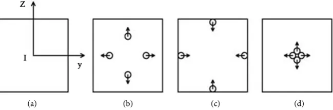
(a) (b) (c) (d)

Figure 3. The three successive characteristic states of the particles of proposed model, within the plane Ixy (a) of the container; (b) Initial state; (c) Impacts of particles on con-tainer walls; (d) Inter-particle collisions in the central region of the concon-tainer. The arrows represent instantaneous velocities of the particles.

The particles are initially provided with equal speeds directed outwards. And they pass successively through three characteristic states: 1) Initial state (Figure 3(b)). 2) Impacts of particles on container walls (Figure 3(c)), where their speeds are inversed. 3) Inter-particle collisions, in the central region of the con-tainer, where again their speeds are inversed.

Obviously, all the six particles, as they move symmetrically, they pass simul-taneously from the above three characteristic states.

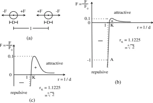
The mutual repulsive forces F between a particle and a container wall (Figure 4(a)) are described by the repulsive part of a Lennard-Jones curve [14] [15] (Figure 4(b)). If the perpendicular distance  of the center of particle from container wall is quite large:

1.1225D 2

≥



where D diameter of particle and 6

1.1225= 2, then

0,

F

=

that is no force F is developed between the particle and the wall. On the contrary, if  is quite small:

1.1225D 2 ,

<



a mutual repulsive force F is developed between particle and wall, given by the equation (Figure 4(b)):

0 13 7

2 1

F F

r r

 

= _− + _

  (1)

where

2 r

D

=  _{and the determination of force coefficient F0 of Lennard-Jones}

curve is described in the following Section 4.1.

The mutual forces F, attractive or repulsive, between any couple of particles, with a distance  of their centers (Figure 5(a)), are described by the Len-nard-Jones curve of Figure 5(b). In Figure 5(c) is shown enlarged the attractive part of this Lennard-Jones curve, because of the significance of attractive forces.

(a) (b)

Figure 4. (a) Perpendicular distance  of a particle from container wall and mutual re-pulsive force F between particle and wall; (b) Repulsive part of a Lennard-Jones curve de-scribing the function F

( )

Figure 5. (a) Distance  and mutual inter-particle force F, attractive (+) or repulsive (−), between a couple of particles; (b) Lennard-Jones curve describing the function

( )

F  ; (c) The Lennard-Jones curve with enlarged its attractive part.

0 13 7

2 1

,

F F

r r

 

= _− + _

  (2)

where r= D.

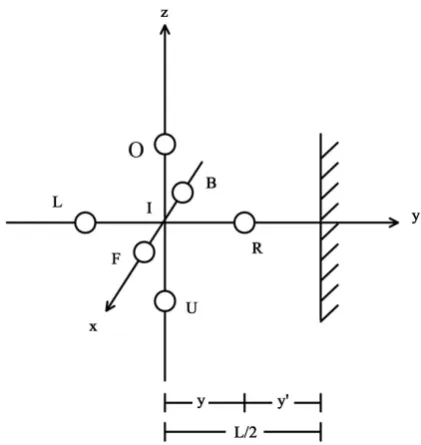
Thanks to the symmetrical movement of all the six particles, it is enough to study the movement of only one particle, let choose that on right part of axis Iy of Figure 2 and name it R (right), as shown in Figure 6. If the distance of this particle from container wall at right is quite small y′ = < 1.1225D 2, then the mutual particle-wall repulsive force is activated, according to Figure 4 and equ-ation (1), and let call this force Fw.

At left of Figure 6, the particle R interacts with the other five particles of the model. The relative position of point R under consideration with respect to four of these particles, F, B, O, U (front, back, over, under) is symmetric. So, the ho-rizontal resultant F4 of the four equal forces (attractive or repulsive), by which the points F, B, O, U act on point R is, according to Figure 5 and Figure 6 and Equation (2):

(a)

(b)

Figure 6. The particle R under consideration is moving on axis Iy. At right, it reaches up to impact with container wall. At left, it interacts with all the other five particles: (F, B, O, U) and L.

4 0 13 7

2 1

4 0.7071 ,

F F

r r

 

= × _− + _

  (3)

where r= D and = y 0.7071D.

Finally, the left particle L acts on particle R, by an, always attractive, force F_, which is given by Figure 5 and Figure 6 and Equation (2), with =2y.

So, the horizontal force on particle R, due to inter-particle action, is

4

i

F =F +F_

and the total horizontal force on particle R, due to inter-particle action and im-pact on wall is,

R i w

F =F +F

and the acceleration of particle R, under consideration, is, at any instant,

(

)

γ = + _.

3. Step-by-Step Algorithm

It has been described, in the previous Section 2, how the proposed model is re-duced, thanks to the symmetric movement of its six particles, to the study of the movement of the single particle R (Figure 6). So, the problem is reduced to the nonlinear dynamic analysis of a SDOF (single degree of freedom) oscillator, which can be solved numerically by a step-by-step time integration algorithm.

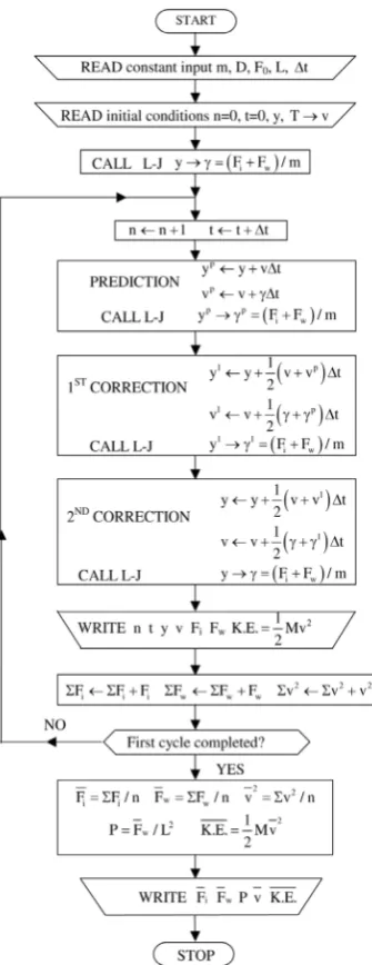
3.1. Flow-Chart

The flow-chart of the proposed algorithm is shown in Figure 7 and is briefly described below.

First, the constant input data are read: particle mass m and diameter D, force coefficient Fo of L-J (Lennard-Jones) curve, side L of cubic container, time

step-length ∆t of the algorithm.

The initial conditions are read: position y, temperature T and speed v of the particle R under consideration. The initial speed v results from initial tempera-ture T, by a thermodynamic postulate, which will be described in following sec-tion 4.1.

The subroutine L-J (Lennard-Jones) is called, which, from the initial position y of the particle, determines the initial forces Fi and Fw, acting on it, and its

initial acceleration γ =

(

)

Within each step of the algorithm, first the steps counter n is increased by 1 and time t by ∆t.

Then, the prediction is performed, which determines the predicted values ,

p p

y v of state variables and the subroutine L-J is called, which, from the given

p

y determines the predicted acceleration γp.

The first correction, by trapezoidal rule, determines the first corrections

1 1

,

y v of the state variables. The subroutine L-J, from y1, finds the first correc-tion of acceleracorrec-tion γ1.

The second and final correction finds the final values of y v, , for present step, and the subroutine L-J, from y, determines the final forces Fi, Fw and

accele-ration γ, for present step.

The output, of present step of algorithm, is printed: steps counter n, time t, position y and speed v of the particle, forces Fi due to inter-particle action and

w

F due to impact on wall, instantaneous total kinetic energy, for all six particles

2

. . 1 2

K E = Mv , where M = 6 m.

At the end of step of algorithm, three summations are made: The present force

i

F, due to inter-particle action, is summed to

∑

impact on wall is summed to

∑

2 v is summed to 2

v

∑

Then, if the first cycle of oscillation has not yet been completed, we continue with the next step of the algorithm.

When the first cycle of oscillation is completed, by returning to the initial state, if we continued the algorithm, everything would be repeated the same, with only a small algorithmic damping. So, the algorithm is interrupted and the global output data are printed, which are:

1)Mean inter-particle force Fi =

∑

2)Mean particle-wall impact force Fw=

∑

It results Fi ≈ −Fw, as is due for global equilibrium.

3)Pressure on wall 2

w

P=F L , in Pascals = N/m2, which, divided by 101,325 N/m2_{, turns to atm units.}

4)Mean 2nd power of speed 2 2

v =

∑

( )

which, for small molar volumes, results significantly lower than the initial speed.

5)Mean total kinetic energy 1 2

. . 2

K E = M v in Joules = N⋅m.

3.2. Computer Program

The program is written in the version Force 2.0 of Fortran, whose compiler is free available, even in Internet cafés.

4. Applications

The proposed simplified coarse-grained dynamic model for real gases is applied on Carbon Dioxide (CO2), which exhibits a particular behavior in Critical point region, as it condensates for rather high temperatures, slightly lower than

31 C 304 K

T =  = .

From the next Section 4.1, it is apparent that, in order to calibrate the pro-posed model on other gases, the following data are required: molar mass, in-compressibility limit of molar volume, as well as temperature, pressure and mo-lar volume at the Critical Point.

4.1. Determination of Parameters

The numerical values of parameters of proposed model are determined below, which will be used in the following applications:

1)The mass of a particle is m=M 6=0.044 kgr 6=0.007333 kgr, where M = 0.044 kgr is the molar mass of Carbon Dioxide.

2)The diameter D of a particle is determined on the basis of criterion of in- compressibility of closely-packed equal spherical particles, as shown in Figure 8. According to experimental evidence [14] [16] [20], the in-compressibility limit of molar volume, for Carbon Dioxide, is about V = 50 cm3_{, which} cor-responds to a cubic container with side L = 3.684 cm. In Figure 8, the spheri-cal particles of proposed model are shown, closely -packed in such a small container. The inter-particle distances are 1.1225D and the particle-wall dis-tances are 1.1225D/2, as, for smaller distances, mutual repulsive forces begin to develop (see Figure 4 and Figure 5). So, on the basis of configuration of Figure 8, the following inequality must be valid:

(

)

D + × <

from which

1.3594 cm D<

and a value D = 1.35 cm is chosen.

3)The force coefficient Fo of Lennard-Jones curve (Equations (1) and (2)) is

determined by calibration of proposed model on the Critical point of Carbon Dioxide. For a cubic container with the critical volume _{94 cm}3

c

V = , that is

4.55 cm

c

L = and for the critical temperature Tc =31 C =304 K, according to test data [14] [16] [20], various values of Fo are tried, until to achieve a

value of pressure, with satisfactory approximation to the experimental critical pressure of CO2, Pc =72.8 atm. In this way, a value Fo =675 kN is obtained.

Application on Critical point is described in Section 4.5.

4)For the side L of cubic container, in STP (standard temperature-pressure) conditions, the value L=28.195 cm is chosen, which corresponds to a vo-lume V = 22.414 liters. And, in the Critical point region of CO2, values of L ranging from 4.0cm up to 9.0 cm are used, which correspond to container vo-lumes V = L3 _{ranging from 64 cm}3 _{up to 729 cm}3_.

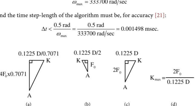
5)The time step-length ∆t of the proposed step-by-step integration algorithm can be determined on the basis of the accuracy criterion of the algorithm [21],

max t 0.5 rad

ω ∆ <

where 2

max Kmax m

ω = .

A maximum stiffness Kmax appears in two cases: inter-particle collision (Figure 5 and Figure 6 and Equation (3)) and particle-wall impact (Figure 4 and Equation (1)). By linearization of branch AK in the Lennard-Jones curves in Figure 4(b) and Figure 5(b), the stiffness of the above two cases can be deter-mined on the basis of Figure 9(a) and Figure 9(b), respectively. It is observed that both give the same value of stiffness, represented by Figure 9(c), which is

6 2

max

2 675 kN

2 0.1225 816.4 10 kgr sec

0.1225 0.0135 cm

o

K = F D= × = ×

×

So,

6 2

2 max 11 2 2

max

816.4 10 kgr sec

1.113 10 rad sec , 0.007333 kgr

K m

ω = = × = ×

max 333700 rad sec

ω =

and the time step-length of the algorithm must be, for accuracy [21]:

max

0.5 rad 0.5 rad

0.001498 msec. 333700 rad sec

t

ω

∆ < = =

(a) (b) (c) (d)

However, the cost, from using a further shorter time step-length ∆t of the algorithm, is negligible, as the computing time, for the first oscillation cycle of the model, is only a few seconds. So, a _{∆ =t 10}−4_msec is chosen, much shorter

than that required by the above accuracy criterion of the algorithm, so that to achieve more accuracy.

6)The initial position of the particle R under consideration is y0 =L 4, where L side of cubic container, as mentioned in Section 2 and according to Figure 2 and Figure 6.

7)Initial temperatures, ranging from T0 = −50 C =223 K in liquid phase re-gion up to T0 =100 C =373 K in gas phase region, are used.

8)The initial speed v0, of the particle under consideration, is obtained from the initial temperature T0, by the thermodynamic postulate:

(

)

0 3 0 ,

v = RT M

where R = 8.3144 Joules−1_∙K−1 _{is the value of gas constant for ideal gases.} How-ever, for small molar volumes, through the oscillation of the particle, the speed v

is significantly reduced, which implies mean values of R much smaller than the initial one, as will be shown in the applications.

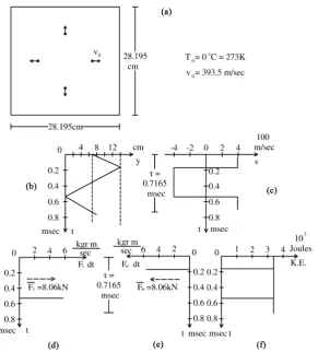
4.2. First Application. STP Conditions. Ideal Gas

A mole of Carbon Dioxide is considered, within a cubic container of side L = 28.195 cm, that is volume _{V =L}3_{=22.414 liters}, with an initial temperature

0 0 C 273 K

T =  = , thus an initial speed of the particle

(

)

1

0 3 8.3144 Joules K 273 K 0.044 kgr 393.5 m sec.

v = × ⋅ − × =

In this first application, point particles are assumed, that is with zero volume, and the inter-particle attractive forces are ignored. So, we have an ideal gas. This case is simple, so it will be solved by hand.

Within the first cycle of oscillation, the particle, starting from the position

0 4

y =L (Figure 6), goes to impact on wall at right, where the speed is re-versed. Then, an inter-particle collision occurs at left, where the speed is again reversed and the particle returns to the initial position. So, the particle runs twice the distance L/2 (Figure 6), with the constant speed v = 393.5 m/sec and the period of oscillation is

2 2 0.28195 m

0.7165 msec. 393.5 m sec

L L

v v

τ = = = =

In Figure 10(a), a sketch of the large container, with the point particles (of zero volume), in the initial state is shown, with the speeds directing outwards. In Figures 10(b)-(f), for the first oscillation cycle, the variations, with respect to time t, of five quantities, are presented: (b). Position y of the particle. (c). Speed v. (d). Inter-particle impulse F dti . (e). Particle-wall impulse F dtw . (f). Total

ki-netic energy, for all six particles,

2

. . 1 2 K E = Mv

Figure 10. First application. STP conditions. Ideal gas. (a) Large container of side L = 28.195 cm with point-particles in the initial state. In the following diagrams, variations of five quantities, with respect to time t; (b) Position y of the particle; (c) Speed v; (d) In-ter-particle impulse F dti ; (e) Particle-wall impulse F dtw ; (f) Total kinetic energy

2

. . 1 2

K E = Mv .

At inter-particle collision and particle-wall impact, the impulse-momentum conservation equation can be written:

2 2 0.007333 kgr 393.5 m sec 5.771 kgr m sec

i w

F dt= −F dt= ∆ =m v mv= × × = ⋅

Here,

dt

→

0

above impulses by the period τ:

3

5.771 kgr m sec

2 8.055 kN

0.7165 10 sec

i w

F = −F = mvτ = ⋅ ₋ =

×

where Fi, Fw are opposite, as is due for equilibrium, and are noted in Figure

10(d) and Figure 10(e), respectively. The pressure on the wall is

2

2 2

8.055 N

101.320 Pascal 1.0 atm. 0.28195 m

w

P=F L = = ≈

as was expected for an ideal gas in STP conditions.

2 2 2

1 1

. . 0.044 kgr 393.5 m sec 3406.5 Joules

2 2

K E = Mv = × =

The potential energy is

2 3

3 3

. . 101.320 N m 0.022414 m 3406.5 Joules

2 2

P E = PV = × =

and the thermodynamic quantity is

1

3 3

8.3144 Joules K 273.15 K 3406.5 Joules. 2RT 2

−

= ⋅ × =

It is observed that . . . . 3 , 2

K E =P E = RT as is due for an ideal gas. That is, the

proposed model describes accurately the behavior of an ideal gas.

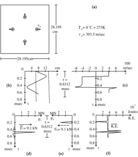
4.3. Second Application. STP Conditions. Real Gas

The same input data, of the previous first application, in STP conditions, are again considered, that is a cubic container with side L = 28.195 cm, thus volume

3 _{22.414 liters}

V =L = , and initial temperature T0=0 C =273 K, thus initial speed of the particle v0=393.5 m sec. However, now, the volume of particles, with diameter D = 1.35 cm, and the inter-particle attractive forces, described by a Lennard-Jones curve (Figure 5, Equation (2)), with a force coefficient

0 675 kN

F = , are taken into account. So, we have a real gas, and the proposed step-by-step time integration algorithm is used, in order to follow the oscillation of the particle.

In Figure 11(a), is shown the large container of side L = 28.195 cm, with the particles of diameter D = 1.35 cm, in the initial conditions. In the Figures 11(b)-(f), are presented, within the first oscillation cycle, the variations, with respect to time t, of five quantities: b) position y of the particle. c) speed v. d) in-ter-particle force Fi. e) particle-wall force Fw. f) total kinetic energy

2

. . 1 2

K E = Mv , n = 6312 steps of the algorithm have been performed, within the first oscillation cycle, with a time-steplength 4

10 msec

t −

∆ = _{, thus the period is}

0.6312 msec

τ

The mean inter-particle force is

57620 N 6312 9.128 kN

i i

F =

∑

and the mean particle-wall force

57080 N 6312 9.050 kN

w w

F =

∑

It is observed that Fi ≈ −Fw, as is due for global equilibrium. The mean forces

i

F, F_w are noted in the Figure 11(d) and Figure 11(e), respectively. The pressure on the wall is

2 _{9.050 10 N 0.28195 m}6 2 2 _{113840 Pascal 1.123 atm 1.0 atm}

w

P=F L = × = = >

that is, it slightly deviates from the ideal gas value. The mean 2nd _{power of speed is}

6 2 2

2 2 1.002 10 m sec 2 2

158750 m sec 6312

Figure 11. Second application. STP conditions. Real gas. (a) Large container of side L = 28.195 cm with particles of diameter D = 1.35 cm, in the initial state. In the following diagrams, variations of five quantities with respect to time t; (b) Position y of the particle; (c) Speed v; (d) Inter-particle force Fi; (e) Particle-wall force Fw; (f) Total kinetic

en-ergy 2

. . 1 2

K E = Mv .

So, the mean (rms) speed is

( )

(

)

1 2 2

0

158750 398.4 m sec 393.5 ,

v= v = = > =v

that is, slightly larger than initial speed. And the mean kinetic energy is

2 2 2 2

1 1

. . 0.044 kgr 398.4 m sec 3491.9 Joules 3406.5,

2 2

K E = Mv = × = >

that is, it slightly deviates from the corresponding value of ideal gas. The mean kinetic energy is noted on the diagram K.E.-t of Figure 11(f), for comparison.

4.4. Third Application. Condensation for Small Molar Volume

A small cubic container with side L = 4.55 cm, thus molar volume

3 3

94 cm

V =L = , is considered, the same as in the Critical point of Carbon Dio-xide, according to test data [14]. And a low initial temperature T0 = −50 C =223 K, which implies a low initial speed of the particle

(

)

1

0 3 8.3144 Joules K 223 K 0.044 kgr 355.6 m sec.

v = × ⋅ − × = A sketch of the

Figure 12. Third application. Condensation for small molar volume. (a) Small container of side L = 4.55 cm with particles of diameter D = 1.35 cm, in the initial state. In the fol-lowing diagrams, variations of four quantities, with respect to time t; (b) Position y of the particle; (c) Speed v; (d) Inter-particle force Fi; (e) Total kinetic energy

2

. . 1 2

K E = Mv .

The application run by the proposed step-by-step algorithm, with

4

10 msec

t −

∆ = . The first oscillation cycle was completed in 475 steps, thus the period is

τ

In Figures 12(b)-(e), the variations, with respect to time t, of four quantities, are presented: b) position y of the particle. c) speed v. d) inter-particle force Fi.

e) total kinetic energy _{K E. .=1 2Mv}2_.

In the present application, because of the low initial temperature, thus low ini-tial speed and kinetic energy, too, the inter-particle attractive forces Fi

over-come the kinetic energy of the particle, thus preventing it from reaching to im-pact on the wall. So zero particle-wall forces Fw =0 and zero pressure P result, which mean that a liquid phase exists.

Because of the zero particle-wall forces, Fw =0, the sum of inter-particle forces results zero,

∑

The mean 2nd _{power of speed results}

2 2

2 2 23368000 m sec 2 2

49196 m sec , 475

v =

∑

2 2 2

. . 1 2 0.044 kgr 221.8 m sec 1082 Joules,

K E = × × =

which is noted on the diagram K.E.-t of Figure 12(e), for comparison.

4.5. Fourth Application. Critical Point

The same small cubic container of side L = 4.55 cm of previous application is considered, which implies a volume 3 _{94 cm ,}3

c

V =L = known, from experiments, as the critical molar volume of Carbon Dioxide [14]. And the initial critical temperature Tc =31 C =304 K is provided, which implies an initial particle speed

(

)

0 3 8.3144 Joule K 304 K 0.044 kgr 415.1 m sec.

v = × ⋅ − × =

In Figure 13(a), a sketch of the above small container, of side L = 4.55 cm, is shown, with the particles of diameter D = 1.35 cm, in the initial state, with the speeds directed outwards.

Figure 13. Fourth application. Critical point. (a) The small container of side L = 4.55 cm with particles of diameter D = 1.35 cm, in the initial state. In the following diagrams, variations of five quantities with respect to time t; (b) Position y of the particle; (c) Speed v; (d) Inter-particle force Fi; (e) Particle-wall force Fw; (f) Total kinetic energy

2

. . 1 2

The application run by the proposed step-by-step algorithm, with

4

10 msec.

t −

∆ = _{The first oscillation cycle was completed in 562 steps, so the}

pe-riod is

τ

In Figures 13(b)-(f), the variations, with respect to time t, of five quantities, are presented: b. position y of the particle. c. speed v. d. inter-particle force Fi. e.

particle-wall force Fw. f. total kinetic energy

2

. . 1 2 . K E = Mv

The mean inter-particle force results Fi =

∑

∑

i

F, F_w are noted on the diagrams F_i − t, F_w − t of Figure 13(d) and Figure 13(e), respectively.

The pressure on the wall is

2 2 2 6

6

15.32 kN 0.0455 m 7.400 10 Pascals

7.400 10 101325 73.03 atm,

w

P=F L = = ×

= × =

close to the experimental critical pressure Pc =72.8 atm [14]. The mean 2nd _{power of speed is}

2 2

2 2 33265000 m sec 2 2

59190 m sec . 562

v =

∑

Thus, the mean (rms) speed results

(

)

0

59190 243.3 m sec 415.1 ,

v= = < =v

much smaller than the initial speed. The mean kinetic energy results

2 2 2 2

. . 1 2 1 2 0.044 kgr 243.3 m sec 1302 Joules,

K E = Mv = × × =

which is noted on the diagram K.E.-t of Figure 13(f), for comparison.

The above mean kinetic energy K E. . corresponds to a value of gas constant

R = 2.856 Joules mole−1_∙K−1_{, as obtained by equating 1302 Joules=3 2R×304 K.} The present value of R is much smaller than the value R = 8.3144 of ideal gases. This will be discussed in the fifth application of next section 4.6.

The present application is adapted to the Critical point by its initial tempera-ture T =31 C =304 K, which is the critical temperature of Carbon Dioxide, according to test data [14]. In the fifth application of next Section 4.6. The Criti-cal point of CO2 will be determined in two different ways: By the group of iso- kinetic energy curves of Figure 14 and by the group of iso-therms of Figure 16. Both cases are close to the Critical point of present application.

4.6. Fifth Application. Iso-Kinetic Energy Curves in the

Critical Point Region

For side of cubic container ranging from L = 4.0 cm up to 9.0 cm, with a step 0.2 cm

L

∆ = _{, that is, volume V = L}3 _{ranging from 64 cm}3 _{up to 729 cm}3_{. And for} initial temperature ranging from T0 = −50 C =223 K up to 100 C =273 K, with a step ∆ =T 10 C =10 K, thus, for initial speed ranging from

0 355.6 m sec

Figure 14. Fifth application. Iso-kinetic energy curves

(

)

. . 1 2 ,

K E = Mv in the Critical

Point region of Carbon Dioxide obtained by the proposed model. C.P. = Critical Point. In the drawning of successive curves, between 1100 and 1400 Joules the step is 50 Joules, between 1400 and 1800 Joules the step is 100 Joules, between 1800 and 3000 Joules the step is 200 Joules.

(V, P) was placed on the volume-pressure plane, with the corresponding K E. . noted on it.

Then, by linear interpolation between successive values of K E. ., iso-kinetic energy curves, for rounded values of K E. ., were obtained, as shown in Figure 14, for K E. . ranging from 1100 Joules up to 3000 Joules.

It is observed that, under the iso-kinetic energy curve of 1100 Joules, a Liquid phase exists, with zero pressures. Between the curve of 1100 Joules and the Crit-ical curve of 1300 Joules, a Vapor phase exists with low pressures. And above the Critical curve, a Gas phase exists, with high pressures. That is, the Critical

iso-. iso-.

K E curve of 1300 Joules is the boundary between the Vapor and Gas phases. By placing the above iso-kinetic energy curves of proposed model on the same P-V (pressure-molar volume) plane, together with the corresponding iso-therms of test data of Eastman-Rollefson [14] [20] and those of Van der Waals model [14] [16] and, by equating, at points of intersection of iso-K E. . curves with iso- therms, K E. .=3 2RT, values of gas constant R are obtained. And a variation of R values, in the Critical point region of Carbon Dioxide is revealed. Both, test data of Eastman-Rollefson and results of Van der Waals model exhibit similar trends, as regards this variation.

Figure 15. Variation of gas constant R values in the Critical Point region of Carbon Di-oxide, obtained by comparison of iso-K E. . curves of proposed model of Figure 14 with corresponding iso-therms of Eastman-Rollefson tests [14] [20] and those of Van der Waals model [14] [16].

With the help of this graph, the iso-kinetic energy curves of proposed model, of Figure 14, have been transformed to the iso-therms shown in Figure 16, for temperatures ranging from T = 250 K up to 400 K with a step ∆ =T 10 K.

The above iso-therms of proposed model are compared with corresponding ones of the test data of Eastman-Rollefson [14] [20], in Figure 17, as well as with those of Van der Waals model [14] [16], in Figure 18.

It is observed, in the Figure 17 and Figure 18, that the proposed model better represents the wave-shaped isotherms of the Van der Waals model, in the Vapor region, than the horizontal linear isotherms of the test data by Eastman–Rollef- son. Also, the proposed model approximates better the larger incompressibility limit of the molar volume given by the Van der Waals model (Figure 18), than the smaller one of the test data by Eastman-Rollefson (Figure 17).

5. Conclusions

A simplified coarse-grained dynamic model, for real gases, is proposed. Five ap-plications of this model, on Carbon Dioxide, are presented:

1)In STP conditions, by ignoring particle volume and inter-particle attractive forces, the proposed model accurately represents the behavior of an ideal gas. 2)Again in STP conditions, but taking into account the particles volume and

in-ter-particle attractive forces, the proposed model slightly deviates from the behavior of an ideal gas, as was expected.

Figure 16. Iso-therms of proposed model in Critical Point region of Carbon Dioxide, ob-tained from transformation of iso-K E. . curves of proposed model of Figure 14, by use of variation of gas constant R values of Figure 15. C.P.: Critical Point.

Figure 17. Comparison of iso-therms of proposed model to corresponding ones of East-man-Rollefson tests [14] [20], in the Critical Point region of Carbon Dioxide.

4)At the Critical point of Carbon Dioxide, the proposed model closely predicts the values of critical molar volume, temperature and pressure, known from experiments [14].

5)Iso-kinetic energy curves have been determined, by the proposed model, in the Critical point region of Carbon Dioxide. By comparing these iso-kinetic energy curves to corresponding iso-therms of test data by Eastman-Rollefson [14] [20] and to those of Van der Waals model [14] [16], a variation of values of gas constant R, in Critical point region, is revealed, ranging from 2.85 up to 5.0 Joules mole−1_∙K−1_{. With the help of this variation of values of R, the} iso-kinetic energy curves of proposed model are transformed to iso-therms, which are compared to corresponding ones of test data by Eastman-Rollefson, as well as to iso-therms of Van der Waals model. And a better agreement is achieved between the proposed model and the Van der Waals model, as shown in Figure 18, as regards a larger in-compressible molar volume and particularly the wave-shaped iso-therms in the Vapor region.

The above five numerical experiments show that the proposed simplified model can approximate the observed behavior of real gases.

In the present work, in order to achieve simplicity, the accuracy is reduced. However, if a refined version of the proposed model, with more particles, is de-veloped, the accuracy can be improved.

References

[1] Müller, E.A. and Jackson, G. (2014) Force-Field Parameters from the SAFT-γ

Equa-tion of State for Use in Coarse-Grained Molecular SimulaEqua-tion. Annual Review of Chemical and Biomolecular Engineering, 5, 405-427.

https://doi.org/10.1146/annurev-chembioeng-061312-103314

[2] Herdes, C., Totton, T.S. and Müller, E.A. (2015) Coarse-Grained Force Field for the Molecular Simulation of Natural Gases and Condensates. Fluid Phase Equilibria 406, 91-100. https://doi.org/10.1016/j.fluid.2015.07.014

[3] Mejía, A., Herdes, C. and Müller, E.A. (2014) Force Fields for Coarse-Grained Mo-lecular Simulations from a Corresponding States Correlation. Industrial & Engi-neering Chemistry Research, 53, 4131-4141. https://doi.org/10.1021/ie404247e

[4] Avendaño, C., Lafitte, T., Galindo, A., Adjiman, C.S., Jackson, G. and Müller, E.A. (2011) Saft-γ Force Field for the simulation of Molecular Fluids. 1. A Single-Site Coarse-Grained Model for Carbon Dioxide. The Journal of Physical Chemistry, 115, 11154-11169. https://doi.org/10.1021/jp204908d

[5] Matteo, B., Oettel, M.M., Yelash, L. and Binder, K. (2009) (SI) Structure and Pair Correlations of a Simple Coarse-Grained Model for Super-Critical Carbon Dioxide. Molecular Physics, 107, 1-24.

[6] Yelash, L., Müller, M., Paul, W. and Binder, K. (2006) How Well Can Coarse- Grained Models of Real Polymers Describe their Structure? The Case of Polybuta-diene. Journal of Chemical Theory and Computation, 2, 588-597.

https://doi.org/10.1021/ct0502099

[7] Theodorakis, P.E., Müller, E.A., Richard, V.K. and Matar. O.K. (2015) Super-spreading: Mechanisms and Molecular Design. Langmuir, 31, 2304-2309.

https://doi.org/10.1021/la5044798

and Structure-Based Coarse-Grained Approaches for the Molecular Dynamics Stu- dies of Conformational Transitions in Proteins. Journal of Chemical Theory and Computations,13, 1366-1374. https://doi.org/10.1021/acs.jctc.6b00986

[9] Kmiecik, S., Gront, D., Kolinski, M., Wieteska, L.A., Dawid, E. and Kolinski, A. (2016) Coarse-Grained Protein Models and Their Applications. Chemical Reviews, 116, 7896-7936. https://doi.org/10.1021/acs.chemrev.6b00163

[10] James, F., Dama, A.V., Sinitskiy, M.C., Weare, J., Roux, B., Aaron, R., Gregory, D. and Voth, A. (2013) The Theory of Ultra-Coarse-Graining. 1. General Principles. Journal of Chemical Theory and Computation, 9, 2466-2480.

[11] Darlyan, A., James, F., Dama, A., Sinitskiy, G. and Voth, A. (2014) The Theory of Ultra-Coarse-Graining. 2. Numerical Implementation. Journal of Chemical Theory and Computation, 10, 5265-5275. https://doi.org/10.1021/ct500834t

[12] James, F., Jaehyeok, D.J. and Voth, G.A. (2017) The Theory of Ultra-Coarse- Graining. 3. Coarse-Grained Sites with Rapid Local Equilibrium of Internal States. Journal of Chemical Theory and Computation, 13, 1010-1022.

[13] Sanghi, T. And Aluru, N.R. (2012) Coarse-Grained Potential Models for Structural Prediction of Carbon Dioxide (CO2) in Confined Environments. The Journal of Chemical Physics, 136, 1-23. https://doi.org/10.1063/1.3674979

[14] Barrow, G.M. (1997) Physical Chemistry. McGraw-Hill, New York. [15] Wikipedia (2017) Lennard-Jones Potential.

[16] Wikipedia (2017) Wan der Waals Equation.

[17] Wikipedia (2017) Maxwell-Boltzmann Distribution.

[18] Dougill, J.W. (1983) Path Dependence and General Theory for the Progressively Fracturing Solid. Proceedings of the Royal Society of London. Series A, Mathemati-cal and PhysiMathemati-cal Sciences, 390, 341-351.

[19] Papadopoulos, P.G. (1984) Biaxial Network Constitutive Model. Journal of Engi-neering Mechanics Division, 110, 449-464.

https://doi.org/10.1061/(ASCE)0733-9399(1984)110:3(449)

[20] Eastman, E.D. and Rollefson. G.K. (1947) Physical Chemistry. Mc Graw-Hill, New York.

[21] Papadopoulos, P.G. (1984) A Simple Algorithm for Nonlinear Dynamic Analysis of Networks. Computers and Structures, 18, 1-8.

Submit or recommend next manuscript to SCIRP and we will provide best service for you:

Accepting pre-submission inquiries through Email, Facebook, LinkedIn, Twitter, etc. A wide selection of journals (inclusive of 9 subjects, more than 200 journals)

Providing 24-hour high-quality service User-friendly online submission system Fair and swift peer-review system

Efficient typesetting and proofreading procedure

Display of the result of downloads and visits, as well as the number of cited articles Maximum dissemination of your research work

Submit your manuscript at: http://papersubmission.scirp.org/