http://wrap.warwick.ac.uk
Original citation:
DeCorte, E. and Pikhurko, Oleg. (2015) Spherical sets avoiding a prescribed set of
angles. International Mathematics Research Notices.
Permanent WRAP url:
http://wrap.warwick.ac.uk/76069
Copyright and reuse:
The Warwick Research Archive Portal (WRAP) makes this work of researchers of the
University of Warwick available open access under the following conditions.
This article is made available under the Creative Commons Attribution 4.0 International
license (CC BY 4.0) and may be reused according to the conditions of the license. For
more details see:
http://creativecommons.org/licenses/by/4.0/
A note on versions:
The version presented in WRAP is the published version, or, version of record, and may
be cited as it appears here.
E. DeCorte and O. Pikhurko (2015) “Spherical Sets Avoiding a Prescribed Set of Angles,” International Mathematics Research Notices, rnv319, 23 pages.
doi:10.1093/imrn/rnv319
Spherical Sets Avoiding a Prescribed Set of Angles
E. DeCorte
1and O. Pikhurko
21
Einstein Institute of Mathematics, Hebrew University of Jerusalem,
Givat Ram Jerusalem 91904, Israel and
2Mathematics Institute and
DIMAP, University of Warwick, Coventry CV4 7AL, UK
Correspondence to be sent to: e-mail: [email protected]
Let X be any subset of the interval [−1,1]. A subset I of the unit sphere inRnwill be calledX-avoidingifu, v∈/Xfor anyu, v∈I. The problem of determining the maximum surface measure of a{0}-avoiding set was first stated in a 1974 note by Witsenhausen; there the upper bound of 1/ntimes the surface measure of the sphere is derived from a simple averaging argument. A consequence of the Frankl–Wilson theorem is that this
fraction decreases exponentially, but until now the 1/3 upper bound for the casen=3 has not moved. We improve this bound to 0.313 using an approach inspired by Delsarte’s
linear programming bounds for codes, combined with some combinatorial reasoning. In
the second part of the paper, we use harmonic analysis to show that, for n≥3, there always exists an X-avoiding set of maximum measure. We also show with an example
that a maximizer need not exist whenn=2.
1 Introduction
Witsenhausen [19] presented the following problem: letSn−1be the unit sphere inRnand
supposeI⊂Sn−1is a Lebesgue measurable set such that no two vectors inI are orthog-onal. What is the largest possible Lebesgue surface measure of I? Let α(n)denote the
supremum of the measures of such setsI, divided by the total measure ofSn−1. The first
Received March 27, 2015; Revised October 13, 2015; Accepted October 14, 2015 c
The Author(s) 2015. Published by Oxford University Press.
This is an Open Access article distributed under the terms of the Creative Commons Attribution License (http://creativecommons.org/licenses/by/4.0/), which permits unrestricted reuse, distribution, and reproduction in any medium, provided the original work is properly cited.
at University of Warwick on January 28, 2016
http://imrn.oxfordjournals.org/
upper bounds forα(n)appeared in [19], where Witsenhausen deduced that α(n)≤1/n. Frankl and Wilson [10] proved their powerful combinatorial result on intersecting set
systems, and as an application they gave the first exponentially decreasing upper bound α(n)≤(1+o(1))(1.13)−n. Raigorodskii [15] improved the bound to (1+o(1))(1.225)−n using a refinement of the Frankl–Wilson method. Gil Kalai conjectured in his weblog
[11] that an extremal example is to take two opposite caps, each of geodesic radiusπ/4;
if true, this implies thatα(n)=(√2+o(1))−n.
Besides being of independent interest, the aboveDouble Cap Conjectureis also
important because, if true, it would imply new lower bounds for the measurable
chro-matic number of Euclidean space, which we now discuss.
Let c(n) be the smallest integer k such that Rn can be partitioned into sets
X1, . . . ,Xk, withx−y2=1 for each x,y∈Xi, 1≤i≤k. The number c(n)is called the
chromatic number of Rn, since the sets X
1, . . . ,Xk can be thought of as color classes for a proper coloring of the graph on the vertex setRn, in which we join two points
with an edge when they have distance 1. Frankl and Wilson [10, Theorem 3] showed
thatc(n)≥(1+o(1))(1.2)n, proving a conjecture of Erd ˝os thatc(n)grows exponentially. Raigorodskii [16] improved the lower bound to(1+o(1))(1.239)n. Requiring the classes
X1, . . . ,Xkto be Lebesgue measurable yields themeasurable chromatic number cm(n).
Clearly, cm(n)≥c(n). Remarkably, it is still open if the inequality is strict for at least one n, although one can prove better lower bounds on cm(n). In particular, the
expo-nent in Raigorodskii’s bound was recently beaten by Bachoc et al. [3], who showed that
cm(n)≥(1.268+o(1))n. If the Double Cap Conjecture is true, then cm(n)≥(√2+o(1))n because, as it is not hard to show, cm(n)≥1/α(n) for every n≥2. Note that the best known asymptotic upper bound on cm(n)(as well as onc(n)) is (3+o(1))n, by Larman and Rogers [13].
Despite progress on the asymptotics of α(n), the upper bound of 1/3 for α(3)
has not been improved since the original statement of the problem in [19]. Note that
the two-cap construction givesα(3)≥1−1/√2=0.2928· · ·. Our first main result is that α(3) <0.313. The proof involves tightening a Delsarte-type linear programming upper bound (see [2,5,7,8]) by adding combinatorial constraints.
LetLbe theσ-algebra of Lebesgue surface measurable subsets ofSn−1, and letλ
be the surface measure, for simplicity normalized so thatλSn−1=1. For X⊂[−1,1], a subset I⊂Sn−1will be calledX-avoidingifξ, η∈/Xfor allξ, η∈I, whereξ, ηdenotes
the standard inner product of the vectorsξ, η. The corresponding extremal problem is
to determine
αX(n):=supλ (I):I∈L,I is X-avoiding. (1)
at University of Warwick on January 28, 2016
http://imrn.oxfordjournals.org/
For example, ift∈(−1,1)and X=[−1,t), then I⊂Sn−1is X-avoiding if and only
if its geodesic diameter is at most arccos(t). Thus Levy’s isodiametric inequality [14]
shows thatαXis given by a spherical cap of the appropriate size.
A priori, it is not clear that the value ofαX(n)is actually attained by some
mea-surable X-avoiding set I (so Witsenhausen [19] had to use supremum to define α(n)).
We prove in Theorem8.6that the supremum is attained as a maximum whenevern≥3. Remarkably, this result holds under no additional assumptions whatsoever on the setX.
However, in a sense, only closed sets Xmatter: our Theorem9.1shows thatαX(n)does
not change if we replaceXby its closure. Whenn=2, the conclusion of Theorem8.6fails; that is, the supremum in (1) need not be a maximum: an example is given in Theorem3.2. Besides also answering a natural question, the importance of the attainment
result can also be seen through the historical lens: in 1838, Jakob Steiner tried to prove
that a circle maximizes the area among all plane figures having some given perimeter.
He showed that any non-circle could be improved, but he was not able to rule out the
possibility that a sequence of ever-improving plane shapes of equal perimeter could
have areas approaching some supremum which is not achieved as a maximum. Only 40
years later in 1879 was the proof completed, when Weierstrass showed that a maximizer
must indeed exist.
The layout of the paper will be as follows. In Section 2, we make some general
definitions and fix notation. In Section3, we prove a simple and general proposition
giving combinatorial upper bounds for αX(n); this is basically a formalization of the
method used by Witsenhausen [19] to obtain the α(n)≤1/nbound. We then apply the proposition to calculateαX(2)when|X| =1. In Section5, we deduce linear programming upper bounds forα(n), in the spirit of the Delsarte bounds for binary [7] and spherical [8]
codes. We then strengthen the linear programming bound in then=3 case in Section6 to obtain the first main result. In Section8, we prove that the supremumαX(n)is a
max-imum whenn≥3, and in Section9, we show thatαX(n)remains unchanged when X is replaced with its topological closure. In Section10, we formulate a conjecture
general-izing the Double Cap Conjecture for the sphere inR3, in which other forbidden inner
products are considered.
2 Preliminaries
Ifu, v∈Rnare two vectors, their standard inner product will be denoted byu, v. All vectors will be assumed to be column vectors. The transpose of a matrix Awill be
denotedAt. We denote bySO(n)the group ofn×nmatricesAoverRhaving determinant
at University of Warwick on January 28, 2016
http://imrn.oxfordjournals.org/
1, for which AtAis equal to the identity matrix. We will think of SO(n) as a compact
topological group, and we will always assume its Haar measure is normalized so that
SO(n)has measure 1. We denote bySn−1the set of unit vectors inRn,
Sn−1=x∈Rn:x,x =1,
equipped with its usual topology. The Lebesgue measureλon Sn−1is always taken to be
normalized so thatλ(Sn−1)=1. Recall that the standard surface measure ofSn−1is
ωn= 2πn/2
Γ (n/2), (2)
where Γ denotes Euler’s gamma-function. The Lebesgue σ-algebra on Sn−1 will be
denoted byL. When(X,M, μ)is a measure space and 1≤p<∞, we use
Lp(X)=
f: fis anR-valuedM-measurable function and
|f|pdμ <∞
.
For f∈Lp(X), we define f p:=
|f|pdμ1/p. Identifying two functions when they agreeμ-almost everywhere, we makeLp(X)a Banach space with the norm ·
p. The expectation of a function f of a random variable X will be denoted by EX[f(X)], or justE[f(X)]. The probability of an event Ewill be denoted byP[E].
When Xis a set, we use 1Xto denote its characteristic function; that is 1X(x)=1 ifx∈X, and 1X(x)=0,otherwise.
IfG=(V,E)is a graph, a setI is calledindependentif{u, v}∈/Efor anyu, v∈I. Theindependence numberα(G)ofGis the cardinality of a largest independent set inG.
We defineαX(n)as in (1), and for brevity, we letα(n)=α{0}(n).
3 Combinatorial Upper Bound
Let us begin by deriving a simple “combinatorial” upper bound for the quantityαX(n).
Proposition 3.1. Letn≥2 andX⊂[−1,1]. For a finite subsetV⊂Sn−1, we letH=(V,E)
be the graph on the vertex setV with edge set defined by putting{ξ, η} ∈Eif and only if
ξ, η ∈X. ThenαX(n)≤α(H)/|V|.
Proof. Let I⊂Sn−1be anX-avoiding set, and take a uniformO∈SO(n). Let the random
variableYbe the number ofξ∈V with Oξ∈I. Since Oξ∈Sn−1is uniformly distributed
for everyξ∈V, we have by the linearity of expectation thatE(Y)= |V|λ(I). On the other hand,Y≤α(H)for every outcomeO. Thusλ(I)≤α(H)/|V|.
at University of Warwick on January 28, 2016
http://imrn.oxfordjournals.org/
We next use Proposition3.1to find the largest possible Lebesgue measure of a
subset of the unit circle inR2in which no two points lie at some fixed forbidden angle.
Theorem 3.2. Let X= {t}and putγ=arccos2π t. Ifγ is rational andγ=p/q with pandq
coprime integers, then
αX(2)= ⎧ ⎨ ⎩
1/2, ifqis even,
(q−1) / (2q) , ifqis odd.
In this case, αX(2) is attained as a maximum. Ifγ is irrational, then αX(2)=1/2, but there exists no measurableX-avoiding setI⊂S1withλ(I)=1/2.
Proof. Write α=αX(2), and identify S1 with the interval [0,1) via the map
(cosx,sinx)→x/2π. We regard [0,1)as a group with the operation of addition modulo 1. Note thatI⊂[0,1)is X-avoiding if and only if I∩(γ +I)= ∅. This implies immediately thatα≤1/2 for all values oft.
Now supposeγ=p/qwith pandqcoprime integers, and suppose thatqis even. Let S be any open subinterval of [0,1) of length 1/q, and define T: [0,1)→[0,1) by
T x=x+γ mod 1. Using the fact that p and q are coprime, one easily verifies that
I=S∪T2S∪ · · · ∪Tq−4S∪Tq−2Shas measure 1/2. Also I is X-avoiding since T I=T S∪
T3S∪ · · · ∪Tq−3S∪Tq−1Sis disjoint fromI. Thereforeα=1/2.
Next suppose thatqis odd. With notation as before, a similar argument shows
that I∪T2I∪ · · · ∪Tq−3I is an X-avoiding set of measure (q−1)/(2q), and
Proposi-tion3.1shows that this is largest possible, since the pointsx,T x,T2x, . . . ,Tq−1xinduce
aq-cycle.
Finally, suppose thatγ is irrational. By Dirichlet’s approximation theorem, there
exist infinitely many pairs of coprime integers pandq such that |γ−p/q|<1/q2. For
each such pair, let ε=ε(q)= |γ −p/q|. Using an open interval S of length 1q−ε and applying the same construction as above withT defined by T x=x+p/q, one obtains an X-avoiding set of measure at least((q−1)/2)(1/q−ε)=1/2−o(1). Alternatively, the lower boundα≥1/2 follows from Rohlin’s tower theorem [12, Theorem 169] applied to the ergodic transformationT x=x+γ. Thereforeα=1/2.
However, this supremum can never be attained. Indeed, if I⊂[0,1) is an
X-avoiding set with λ(I)=1/2 and T is defined by T x=x+γ, then I∩T I= ∅ and
T I∩T2I= ∅. Since λ(I)=1/2, this implies that I and T2I differ only on a nullset,
contradicting the ergodicity of the irrational rotationT2.
at University of Warwick on January 28, 2016
http://imrn.oxfordjournals.org/
4 Gegenbauer Polynomials and Schoenberg’s Theorem
Before proving the first main result, we recall the Gegenbauer polynomials and
Schoen-berg’s theorem from the theory of spherical harmonics. For ν >−1/2, define the
Gegenbauer weight function
rν(t):=1−t2ν−1/2, −1<t<1.
To motivate this definition, observe that if we take a uniformly distributed vectorξ∈
Sn−1,n≥2, and project it to any given axis, then the density of the obtained random vari-ableX∈[−1,1] is proportional tor(n−2)/2, with the coefficient
1
−1r(n−2)/2(x)dx
−1
=ωn−1
ωn ,
whereωnis as in (2). (In particular,Xis uniformly distributed in [−1,1] ifn=3.)
Applying the Gram–Schmidt process to the polynomials 1,t,t2, . . .with respect to the inner productf,gν=1−1 f(t)g(t)rν(t)dt, one obtains the Gegenbauer polynomials Ciν(t),i=0,1,2, . . ., whereCiνis of degreei. For a concise overview of these polynomials, see, for example, [4, Section B.2]. Here, we always use the normalizationCiν(1)=1.
For a fixedn≥2, a continuous function f: [−1,1]→Ris calledpositive definite, if for every set of distinct pointsξ1, . . . , ξs∈Sn−1, the matrix(f(ξi, ξj))si,j=1 is positive semidefinite. We will need the following result of Schoenberg [17]. For a modern
presen-tation, see e.g. [4, Theorem 14.3.3].
Theorem 4.1(Schoenberg’s theorem). Forn≥2, a continuous function f: [−1,1]→Ris positive definite if and only if there exist coefficientsai≥0, fori≥0, such that
f(t)=
∞
i=0
aiCi(n−2)/2(t) , for allt∈[−1,1].
Moreover, the convergence on the right-hand side is absolute and uniform for every
positive definite function f.
For a given positive definite function f, the coefficients ai in Theorem 4.1are
unique and can be computed explicitly; a formula is given in [4, Equation (14.3.3)].
We are especially interested in the case n=3. Then ν=1/2, and the first few Gegenbauer polynomialsCi1/2(x)are
C01/2(x)=1, C11/2(x)=x, C1/22 (x)=213x2−1,
C31/2(x)=125x3−3x, C41/2(x)=1835x4−30x2+3.
at University of Warwick on January 28, 2016
http://imrn.oxfordjournals.org/
5 Linear Programming Relaxation
Schoenberg’s theorem allows us to set up a linear program whose value upper bounds α(n)forn≥3. The same result appears in [2,5]; we present a self-contained (and slightly simpler) proof for the reader’s convenience. In the next section, we strengthen the linear
program, obtaining a better bound forα(3).
Lemma 5.1. Suppose f,g∈L2Sn−1and definek: [−1,1]→Rby
k(t):=E[f(Oξ)g(Oη)], (3)
where the expectation is taken over randomly chosenO∈SO(n), and ξ, η∈Sn−1are any two points satisfyingξ, η =t. Then,k(t)exists for every−1≤t≤1, andkis continuous.
If f=g, thenkis positive definite.
Proof. The expectation in (3) clearly does not depend on the particular choice of ξ, η∈Sn−1. Fix any pointξ
0∈Sn−1and let P: [−1,1]→SO(n)be any continuous function
satisfyingξ0,P(t)ξ0 =tfor each−1≤t≤1. We have
k(t)=E[f(Oξ0)g(O P(t) ξ0)]. (4)
The functions O→ f(Oξ0) and O→g(O P(t)ξ0) on SO(n) belong to L2(SO(n)); being
an inner product in L2(SO(n)), the expectation (4), therefore, exists for every
t∈[−1,1].
We next show that k is continuous. For each O∈SO(n), let RO:L2(SO(n))→
L2(SO(n)) be the right translation operator defined by (R
OF)(O)=F(OO) for
F∈L2(SO(n)). For fixedF, the mapO→R
OF is continuous fromL2(SO(n))toL2(SO(n)); see e.g. [6, Lemma 1.4.2]. Therefore the functiont→RP(t)F is continuous from [−1,1] to
L2(SO(n)). UsingF(O)=g(Oξ
0), the continuity ofkfollows.
Now suppose f=g; we show that k is positive definite. Let ξ1, . . . , ξs∈Sn−1.
We need to show that thes×smatrix K=(k(ξi, ξj))s
i,j=1 is positive semidefinite. But if v=(v1, . . . , vs)T∈Rsis any column vector, then
vTKv=
s
i=1
s
j=1
E[f(Oξi)fOξj
]vivj=E ⎡ ⎣
s
i=1
f(Oξi) vi
2⎤
⎦≥0.
at University of Warwick on January 28, 2016
http://imrn.oxfordjournals.org/
Theorem 5.2. α(n)is no more than the value of the following infinite-dimensional linear
program:
maxx0
∞
i=0
xi=1
∞
i=0
xiCi(n−2)/2(0)=0
xi≥0, for alli=0,1,2, . . ..
(5)
Proof. Let I∈Lbe a{0}-avoiding subset of Sn−1 withλ(I) >0. We construct a feasible
solution to the linear program (5) having valueλ(I). Letk: [−1,1]→Rbe defined as in (3), with f=g=1I. Thenkis a positive definite function satisfyingk(1)=λ(I)andk(0)=0. By Theorem4.1,khas an expansion in terms of the Gegenbauer polynomials:
k(t)=
∞
i=0
aiCi(n−2)/2(t) , (6)
where eachai≥0 and the convergence of the right-hand side is uniform on [−1,1]. More-over, for each fixedξ0∈Sn−1, we have by Fubini’s theorem and (3) that
Sn−1
k(ξ0, η)dη=
Sn−1
Sn−1
k(ξ, η)dξdη
=E
Sn−1
1I(Oξ)dξ 2
=λ (I)2. (7)
Note that
Sn−1
Ci(n−2)/2(ξ0, η)dη=ωn−1
ωn 1
−1
Ci(n−2)/2(t)1−t2(n−3)/2dt=0
whenever i≥1 by the definition of the Gegenbauer polynomials. Putting (6) and (7) together and using thatC0(n−2)/2≡1, we conclude thata0=λ(I)2.
Recalling that Ci(n−2)/2(1)=1 for i≥0, we find that setting xi=ai/λ(I) for
i=0,1,2, . . .gives a feasible solution of valueλ(I)to the linear program (5).
at University of Warwick on January 28, 2016
http://imrn.oxfordjournals.org/
Unfortunately, in the casen=3, the value of (5) is at least 1/3, which is the same bound obtained when the problem was first stated in [19]. This can be seen from the
feasible solutionx0=1/3,x2=2/3 andxi=0 for alli=0,2.
6 Adding Combinatorial Constraints
For eachξ∈Sn−1and−1<t<1, letσ
ξ,t be the unique probability measure on the Borel subsets ofSn−1whose support is equal to the set
ξt:=η∈Sn−1:η, ξ =t,
and which is invariant under all rotations fixingξ.
Now let n=3. As before, let I∈L be a {0}-avoiding subset of S2 and define
k: [−1,1]→Ras in (3) with f=g=1I; that is,
k(t)=E[1I(Oξ)1I (Oη)],
whereξ, η∈S2satisfyξ, η =t.
Our aim now is to strengthen (5) for the case n=3 by adding combinatorial inequalities coming from Proposition3.1applied to the sections of S2by affine planes.
We proceed as follows. Letpandqbe coprime integers with 1/4≤p/q≤1/2, and let
tp,q=
−cos(2πp/q)
1−cos(2πp/q).
Letξ∈S2be arbitrary. If we take two orthogonal unit vectors with endpoints inξtp,q and the center ξ0=tp,qξ of this circle, then we get an isosceles triangle with side lengths
1−t2
p,q 1/2
and base√2; by the Cosine Theorem, the angle atξ0is 2πp/q.
Let ξ0, η0∈S2 be arbitrary points satisfying ξ0, η0 =tp,q. By Fubini’s theorem, we have
ktp,q
=E[1I(Oξ0)1I(Oη0)]=
ξtp,q 0
E[1I (Oξ0)1I(Oη)]dσξ0,tp,q(η)
=E
1I(Oξ0)
ξtp,q 0
1I(Oη)dσξ0,tp,q(η)
.
But if q is odd, then ξtp,q
0 1I(Oη)dσξ0,tp,q(η)≤
q−1
2q for all O∈SO(n) by Proposition 3.1 applied to the circle (Oξ0)tp,q∼=S1, since the subgraph it induces contains a cycle of
lengthq. Thereforek(tp,q)≤λ(I)q2−q1.
at University of Warwick on January 28, 2016
http://imrn.oxfordjournals.org/
It follows that the inequalities
∞
i=0
xiCi1/2
tp,q
≤(q−1) /2q, (8)
are valid for the relaxation and can be added to (5). The same holds for the inequalities ∞
i=0xiCi1/2(−tp,q)≤(q−1)/2q.
So we have just proved the following result.
Theorem 6.1. α(3)is no more than the value of the following infinite-dimensional linear
program.
maxx0
∞
i=0
xi=1
∞
i=0
xiCi1/2(0)=0
∞
i=0
xiCi1/2
±tp,q
≤(q−1) /2q, forqodd, p,qcoprime
xi≥0, for alli=0,1,2, . . ..
(9)
Rather than attempting to find the exact value of the linear program (9), the idea
will be to discard all but finitely many of the combinatorial constraints, and then to
apply the weak duality theorem of linear programming. The dual linear program has
only finitely many variables, and any feasible solution gives an upper bound for the
value of program (9), and therefore also forα(3). At the heart of the proof is the
veri-fication of the feasibility of a particular dual solution which we give explicitly. While
part of the verification has been carried out by computer in order to deal with the large
numbers that appear, it can be done using only rational arithmetic and can therefore be
considered rigorous.
Theorem 6.2. α(3) <0.313.
at University of Warwick on January 28, 2016
http://imrn.oxfordjournals.org/
Proof. Consider the following linear program:
max
x0: ∞
i=0
xi=1,
∞
i=0
xiCi1/2(0)=0,
∞
i=0
xiCi1/2
t1,3
≤1/3,
∞
i=0
xiCi1/2
t2,5
≤2/5,
∞
i=0
xiCi1/2
−t2,5
≤2/5, xi≥0, for alli=0,1,2, . . .
. (10)
The linear programming dual of (10) is the following.
minb1+
1 3b1,3+
2 5b2,5+
2 5b2,5−
b1+b0+b1,3+b2,5+b2,5−≥1
b1+Ci1/2(0)b0+Ci1/2
t1,3
b1,3+Ci1/2
t2,5
b2,5+Ci1/2
−t2,5
b2,5−≥0 fori=1,2, . . .
b1,b0∈R, b1,3,b2,5,b2,5−≥0. (11)
By linear programming duality, any feasible solution for program (6) gives
an upper bound for (10), and therefore also for α(3). So in order to prove the claim α(3) <0.313, it suffices to give a feasible solution to (6) having objective value no more than 0.313. Let
b=b1,b0,b1,3,b2,5,b2,5−=1016(128614,404413,36149,103647,327177) .
It is easily verified thatbsatisfies the first constraint of (6) and that its objective value is less than 0.313. To verify the infinite family of constraints
b1+Ci1/2(0)b0+C1i/2
t1,3
b1,3+Ci1/2
t2,5
b2,5+Ci1/2
−t2,5
b2,5−≥0 (12)
for i=1,2, . . ., we apply [18, Theorem 8.21.11] (where Ciλ is denoted as Pi(λ)), which implies
|Ci1/2(cosθ)| ≤
√
2
√
π√sinθ
Γ (i+1) Γ (i+3/2)+
1
√π
23/2(sinθ)3/2
Γ (i+1)
Γ (i+5/2) (13)
for each 0< θ < π. Note that t1,3=1/√3 and t2,5=5−1/4. When θ∈A:=
{π/2,arccost1,3,arccost2,5,arccos(−t2,5)}, we have sinθ∈
1,
2 3, γ
, where γ=√2
5+√5.
The right-hand side of Equation (13) is maximized overθ∈Aat sinθ=γfor each fixedi, and since the right-hand side is decreasing ini, one can verify using rational arithmetic
only that it is no greater than 128614/871386=b1/(b0+b1,3+b2,5+b2,5−) wheni≥40,
at University of Warwick on January 28, 2016
http://imrn.oxfordjournals.org/
by evaluating ati=40. Therefore,
b1+Ci1/2(0)b0+Ci1/2
t1,3
b1,3+Ci1/2
t2,5
b2,5+C1i/2
−t2,5
b2,5−
≥b1−
b0+b1,3+b2,5+b2,5−maxθ∈
A C1/2
i (cosθ)
≥0
when i≥40. It now suffices to check that b satisfies the constraints (12) for
i=0,1, . . . ,39. This can also be accomplished using rational arithmetic only.
The rational arithmetic calculations required in the above proof were carried out
withMathematica. When verifying the upper bound for the right-hand side of (13), it is
helpful to recall the identity Γ (i+1/2)=(i−1/2)(i−3/2)· · ·(1/2)√π. When verifying the constraints (12) fori=0,1, . . . ,39, it can be helpful to observe thatt1,3and±t2,5are
roots of the polynomialsx2−1/3 andx4−1/5,respectively; this can be used to cut down
the degree of the polynomialsCi1/2(x)to at most 3 before evaluating them. The ancillary
folder of thearxiv.orgversion of this paper contains aMathematica notebook that
verifies all calculations.
The combinatorial inequalities of the form (8) we chose to include in the
strengthened linear program (10) were found as follows: let L0 denote the linear
pro-gram (5). We first find an optimal solutionσ0toL0. We then proceed recursively; having
defined the linear programLi−1and found an optimal solutionσi−1, we search through
the inequalities (8) until one is found which is violated byσi−1, and we strengthen Li−1
with that inequality to produce Li. At each stage, an optimal solution to Li is found
by first solving the dual minimization problem, and then applying the complementary slackness theorem from linear programming to reduceLi to a linear programming
max-imization problem with just a finite number of variables.
Adding more inequalities of the form (8) appears to give no improvement on the
upper bound. Also adding the constraints ∞i=0xiCi1/2(t)≥0 for −1≤t≤1 appears to give no improvement. A small (basically insignificant) improvement can be achieved by
allowing the odd cycles to embed into S2 in more general ways, for instance with the
points lying on two different latitudes rather than just one.
at University of Warwick on January 28, 2016
http://imrn.oxfordjournals.org/
7 Adjacency Operator
Letn≥3. Forξ∈Sn−1and−1<t<1, we use the notationsξtandσ
ξ,tfrom Section6. For
f∈L2(Sn−1)define A
tf:Sn−1→Rby
(Atf) (ξ):=
ξt
f(η)dσξ,t(η) , ξ∈Sn−1. (14)
Here we establish some basic properties of At which will be helpful later. The
operator At can be thought of as an adjacency operator for the graph with vertex set
Sn−1, in which we join two points with an edge when their inner product ist. Adjacency
operators for infinite graphs are explored in greater detail and generality in [1].
Lemma 7.1. For every t∈(−1,1), At is a bounded linear operator from L2(Sn−1) to
L2(Sn−1)having operator norm equal to 1.
Proof. The right-hand side of (14) involves integration over nullsets of a function
f∈L2(Sn−1) which is only defined almost everywhere, and so strictly speaking one
should argue that (14) really makes sense. In other words, given a particular
representa-tive ffrom itsL2-equivalence class, we need to check that the integral on the right-hand
side of (14) is defined for almost allξ∈Sn−1, and that the L2-equivalence class of A
tf does not depend on the particular choice of representative f.
Our main tool will be Minkowski’s integral inequality; see e.g. [9, Theorem 6.19].
Leten=(0, . . . ,0,1)be thenth basis vector inRnand let
S=(x1,x2, . . . ,xn):xn=0,x12+ · · · +xn2−1=1
be a copy ofSn−2inside Rn. Considering f as a particular measurable function (not an
L2-equivalence class), we defineF :SO(n)×S→Rby
F(ρ, η)= f
ρten+ 1−t2η
, ρ∈SO(n) , η∈S.
Let us formally check all the hypotheses of Minkowski’s integral inequality applied to
F, where SO(n)is equipped with the Haar measure, and where Sis equipped with the
normalized Lebesgue measure; this will show that the functionF˜:SO(n)→Rdefined by
˜
F(ρ)=SF(ρ, η)dηbelongs toL2(SO(n)).
Clearly, the function F is measurable. To see that the function ρ→F(ρ, η)
belongs toL2(SO(n))for each fixedη∈S, simply note that
SO(n)|F(ρ, η)| 2dρ=
SO(n)
f
ρten+ 1−t2η
2
dρ= f22.
at University of Warwick on January 28, 2016
http://imrn.oxfordjournals.org/
That the functionη→ F(·, η)2 belongs to L1(S)then also follows easily (in fact, this
function is constant):
S
SO(n)
|F(ρ, η)|2dρ 1/2
dη=
S
f2dη= f2.
Minkowski’s integral inequality now gives that the function η→F(ρ, η) is in L1(S)
for a.e. ρ, the function F˜ is in L2(SO(n)), and its norm can be bounded as
follows:
˜F2=
SO(n)
SF(ρ, η)dη
2
dρ 1/2
≤
S
SO(n)|F(ρ, η)| 2dρ
1/2
dη= f2. (15)
Applying (15) to f−g,where gis a.e. equal to f, we conclude that theL2-equivalence
class ofF˜ does not depend on the particular choice of representative ffrom its equiva-lence class.
Now (Atf)(ξ) is simply F˜(ρ), where ρ∈SO(n) can be any rotation such that ρen=ξ. This shows that the integral in (14) makes sense for almost allξ∈Sn−1.
We haveAt ≤1 since, for any f∈L2(Sn−1),
Atf2=
Sn−1
|(Atf) (ξ)|2dξ 1/2
=
SO(n)|(Atf) (ρen)| 2dρ
1/2
=
SO(n)
F˜(ρ)2dρ 1/2
≤ f2,
by (15).
Finally, applying Atto the constant function 1 shows thatAt =1.
Lemma 7.2. Let f and g be functions in L2Sn−1, letξ, η∈Sn−1 be arbitrary points,
and writet= ξ, η. IfO∈SO(n)is chosen uniformly at random with respect to the Haar measure onSO(n), then
Sn−1
f(ζ ) (Atg) (ζ )dζ =E[f(Oξ)g(Oη)], (16)
which is exactly the definition ofk(t)from (3).
at University of Warwick on January 28, 2016
http://imrn.oxfordjournals.org/
Proof. We have
Sn−1
f(ζ ) (Atg) (ζ )dζ=
SO(n) f(Oξ) (Atg) (Oξ)dO
=
SO(n) f(Oξ)
(Oξ)tg(ψ)dσOξ,t(ψ)dO,
IfHis the subgroup of all elements inSO(n)which fixξ, then the above integral can be
rewritten as
SO(n) f(Oξ)
H
g(Ohη)dhdO.
By Fubini’s theorem, this integral is equal to
H
SO(n) f(Oξ)g(Ohη)dOdh=
H
SO(n) f
Oh−1ξg(Oη)dOdh
=
SO(n) f(Oξ)g(Oη)dO,
where we use the right-translation invariance of the Haar integral onSO(n)at the first
equality, and the second equality follows by noting that the integrand is constant with
respect toh.
Lemma 7.3. For every t∈(−1,1), the operator At:L2
Sn−1→L2Sn−1 is
self-adjoint.
Proof. Fix ξ, η∈Sn−1 that satisfy ξ, η =t. Lemma 7.2 implies that, for any f,
g∈L2Sn−1, we have
Atf,g =EO∈SO(n)[f(Oξ)g(Oη)]= f,Atg,
giving the required.
8 Existence of a Measurable Maximum Independent Set
Letn≥2 and X⊂[−1,1]. From Theorem3.2, we know that the supremumαX(n)is some-times attained as a maximum, and somesome-times not. It is therefore interesting to ask when
a maximizer exists. The main positive result in this direction is Theorem 8.6, which
says that a largest measurable X-avoiding set always exists when n≥3. Remarkably, this result holds under no additional restrictions (not even Lebesgue measurability)
on the set X of forbidden inner products. Before arriving at this theorem, we shall
need to establish a number of technical results. For the remainder of this section, we
supposen≥3.
at University of Warwick on January 28, 2016
http://imrn.oxfordjournals.org/
For d≥0, letHn
d be the vector space of homogeneous polynomials p(x1, . . . ,xn)
of degreedinnvariables belonging to the kernel of the Laplace operator; that is,
∂2p
∂x2 1
+ · · · + ∂∂2p
x2
n =0.
Note that eachHdnis finite-dimensional. The restrictions of the elements ofHdnto the surface of the unit sphere are called the spherical harmonics. For fixed n, we have
L2(Sn−1)=!∞
d=0Hdn[4, Theorem 2.2.2]; that is, each function in L2
Sn−1 can be
writ-ten uniquely as an infinite sum of elements fromHn
d,d=0,1,2, . . ., with convergence in theL2-norm.
Recall the definition (14) of the adjacency operator from Section7:
(Atf) (ξ):=
ξt
f(η)dσξ,t(η) , f∈L2
Sn−1.
The next lemma states that each spherical harmonic is an eigenfunction of the
operatorAt. It extends the Funk–Hecke formula [4, Theorem 1.2.9] to the Dirac measures,
obtaining the eigenvalues ofAtexplicitly. The proof relies on the fact that integral kernel
operatorsKhaving the form(K f)(ξ)= f(ζ )k(ζ, ξ)dζ for some functionk: [−1,1]→R are diagonalized by the spherical harmonics, and moreover that the eigenvalue of a
spe-cific spherical harmonic depends only on its degree.
Proposition 8.1. Lett∈(−1,1). Then, for every spherical harmonicYdof degreed,
(AtYd) (ξ)=
ξt
Yd(η)dσξ,t(η)=μd(t)Yd(ξ) , ξ∈Sn−1,
whereμd(t)is the constant
μd(t)=Cd(n−2)/2(t)1−t2(n−3)/2.
Proof. Let dsbe the Lebesgue measure on [−1,1] and let {fα}α be a net of functions in L1([−1,1])such that{f
αds} converges to the Dirac point massδt at tin the weak-*
topology on the set of Borel measures on [−1,1]. By [4, Theorem 1.2.9], we have
Sn−1
Yd(η) fα(ξ, η)dη=μd,αYd(ξ) ,
where
μd,α=
1
−1C (n−2)/2 d (s)
1−s2(n−3)/2 fα(s)ds.
By taking limits, we complete the proof.
at University of Warwick on January 28, 2016
http://imrn.oxfordjournals.org/
Lemma 8.2 is a general fact about weakly convergent sequences in a Hilbert
space.
Lemma 8.2. LetHbe a Hilbert space and letK:H→Hbe a compact operator. Suppose
{xi}∞i=1is a sequence inHconverging weakly tox∈H. Then
lim
i→∞K xi,xi = K x,x.
Proof. Let C be the maximum of x and supi≥1xi, which is finite by the Principle of Uniform Boundedness. Let{Km}∞m=1 be a sequence of finite rank operators such that
Km→Kin the operator norm asm→ ∞. Clearly,
lim
i→∞Kmxi,xi = Kmx,x
for each, m=1,2, . . .. Let ε >0 be given and choose m0 so that K−Km0< ε/(3C
2).
Choosingi0so that|Km0xi,xi − Km0x,x|< ε/3 wheneveri≥i0, we have
|K xi,xi − K x,x|
≤ |K xi,xi − Km0xi,xi| + |Km0xi,xi − Km0x,x| + |Km0x,x − K x,x|
≤ K−Km0C
2+ε/3+ K−K
m0C
2< ε,
and the lemma follows.
Corollary 8.3, which is also a result stated in [1], says that the adjacency
opera-tors Atare compact whenn≥3.
Corollary 8.3. Ifn≥3 andt∈(−1,1), then Atis compact.
Proof. The operator At is diagonalizable by Proposition 8.1, since the spherical
har-monics form an orthonormal basis for L2Sn−1. It therefore suffices to show that its eigenvalues cluster only at 0.
By [18, Theorem 8.21.8] and Proposition 8.1, the eigenvaluesμd(t)tend to zero
asd→ ∞. The eigenspace corresponding to the eigenvalueμd(t)is precisely the vector space of spherical harmonics of degreed, which is finite-dimensional. Therefore At is
compact.
For eachξ∈Sn−1, letCh(ξ)be the open spherical cap of heighthinSn−1centered
atξ. Recall thatCh(ξ)has volume proportional to11−h(1−t2)(n−3)/2dt.
at University of Warwick on January 28, 2016
http://imrn.oxfordjournals.org/
Lemma 8.4. For each ξ∈Sn−1, we have λ(Ch(ξ))=Θ(h(n−1)/2) and λ(C
h/2(ξ))≥
λ(Ch(ξ))/2(n−1)/2−o(h(n−1)/2)ash→0+.
Proof. If f(h)=11−h1−t2(n−3)/2 dt, then we have df dh(h)=
2h−h2(n−3)/2. Since
f(0)=0, the smallest power of hoccurring in f(h)is of order(n−1)/2. This gives the first result. For the second, note that the coefficient of the lowest order term in f(h)is
2(n−1)/2times that of f(h/2).
Lemma 8.5. Supposen≥3 and letI⊂Sn−1be a Lebesgue measurable set withλ(I) >0.
Definek: [−1,1]→Rby
k(t):=
Sn−1
1I(ζ ) (At1I) (ζ )dζ,
which, by Lemma7.2, is the same as Definition (3) applied with f=g=1I. Ifξ1, ξ2∈Sn−1
are Lebesgue density points ofI, thenk(ξ1, ξ2) >0.
Proof. Let t= ξ1, ξ2. Ift=1, then the conclusion holds sincek(1)=λ(I) >0. Ift= −1,
thenξ2= −ξ1, and by the Lebesgue density theorem we can choose h>0 small enough
thatλ(Ch(ξi)∩I) >23λ(Ch(ξi))fori=1,2. By Lemma7.2, we have
k(−1)=E[1I(Oξ1)1I(O(−ξ1))]
≥E[1I∩Ch(ξ1)(Oξ1)1I∩Ch(ξ2)(O(−ξ1))]≥
1
3λ (Ch(ξ1)) .
From now on, we may therefore assume −1<t<1. Let h>0 be a small num-ber that will be determined later. Suppose x∈Ch(ξ1). The intersection xt∩Ch(ξ2) is a
spherical cap in the (n−2)-dimensional sphere xt having height proportional to h; this is because Ch(ξ2) is the intersection of Sn−1 with a certain half-space H, and
xt∩Ch(ξ2)=xt∩H. We haveσx,t
xt∩Ch(ξ2)
=Θh(n−2)/2by Lemma8.4, and it follows that there existsD>0 such thatσx,t
xt∩Ch(ξ2)
≤Dh(n−2)/2for sufficiently smallh>0. Ifx∈Ch/2(ξ1), thenxt∩Ch/2(ξ2)= ∅sincextis just a rotation of the hyperplaneξ1t
through an angle equal to the angle betweenxandξ1. Thereforext∩Ch(ξ2)is a spherical
cap inxthaving height at leasth/2.
Thus there exists D>0 such thatσx,t
xt∩Ch(ξ
2)
≥Dh(n−2)/2for all x∈C
h/2(ξ1),
by Lemma8.4.
Now chooseh>0 small enough thatλ(Ch(ξi)∩I)≥
1−2DnD
λ(Ch(ξi))fori=1,2; this is possible by the Lebesgue density theorem sinceξ1 andξ2are density points. We
at University of Warwick on January 28, 2016
http://imrn.oxfordjournals.org/
have by Lemma7.2that
k(t)=P[η1∈I, η2∈I],
ifη1is chosen uniformly at random fromSn−1, and ifη2is chosen uniformly at random
fromηt1. Then
k(t)≥P[η1∈I∩Ch(ξ1) , η2∈I∩Ch(ξ2)]
≥P[η1∈Ch(ξ1) , η2∈Ch(ξ2)]−P[η1∈Ch(ξ1)\I, η2∈Ch(ξ2)]
−P[η1∈Ch(ξ1) , η2∈Ch(ξ2)\I].
The first probability is at least
Dh(n−2)/2λC h/2(ξ1)
≥ D
2(n−1)/2h
(n−2)/2λ (C
h(ξ1))−o
h(2n−3)/2
by Lemma8.4. The second and third probabilities are each no more than
D
2nDλ (Ch(ξ1))Dh
(n−2)/2=D
2nλ (Ch(ξ1))h
(n−2)/2
for sufficiently smallh>0, and therefore, by the first part of Lemma8.4,
k(t)≥ D
2(n−1)/2λ (Ch(ξ1))h
(n−2)/2−oh(2n−3)/2− D
2n−1λ (Ch(ξ1))h
(n−2)/2,
and this is strictly positive for sufficiently smallh>0.
We are now in a position to prove the second main result of this paper.
Theorem 8.6. Suppose n≥3 and let X be any subset of [−1,1]. Then there exists an
X-avoiding set I∈Lsuch thatλ(I)=αX(n).
Proof. We may suppose that 1∈Xfor otherwise everyX-avoiding set is empty and the theorem holds withI= ∅.
Let {Ii}∞i=1 be a sequence of measurable X-avoiding sets such that
limi→∞λ(Ii)=αX(n). Passing to a subsequence if necessary, we may suppose that the sequence{1Ii}of characteristic functions converges weakly inL
2Sn−1; lethbe its limit.
Then 0≤h≤1 almost everywhere since 0≤1Ii≤1 for everyi.
Denote by Ithe seth−1((0,1]), and let I be the set of Lebesgue density points of
I. We claim that I isX-avoiding.
For allt∈X\ {−1}, the operator At:L2(Sn−1)→L2(Sn−1)is self-adjoint and com-pact by Lemma7.3and Corollary8.3. SinceAt1Ii,1Ii =0 for eachi, Lemma8.2implies
at University of Warwick on January 28, 2016
http://imrn.oxfordjournals.org/
Ath,h =0. Sinceh≥0, it follows from the definition of AtthatAt1I,1I =0, and there-fore also thatAt1I,1I =0. But if there exist pointsξ, η∈Iwitht0= ξ, η ∈X\ {−1}, then
At01I,1I>0 by Lemma8.5.
Thus, in order to show that I is X-avoiding, it remains to derive a contradiction
from assuming that−1∈Xand−ξ, ξ∈I for someξ∈Sn−1. Sinceξ and−ξ are Lebesgue
density points of I, there is a spherical capC centered atξ such thatλ(I∩C) >23λ(C)
andλ(I∩(−C)) >32λ(C). The same applies toIifor all largei(since a cap is a continuity set). But this contradicts the fact that Ii and its reflection −Ii are disjoint for every i. ThusI is X-avoiding.
Finally, we have
λ (I)=λI≥ 1Sn−1,h =lim
i→∞1S
n−1,1Ii =lim
i→∞λ (Ii)=αX(n) ,
whenceλ(I)=αX(n)sinceλ(I)≤αX(n).
Note that the proof of Theorem 8.6would fail forn=2, because the adjacency operators At need not be compact; the reason for this is that the eigenvalues μd(t) of
Proposition8.1do not tend to zero asd→ ∞.
9 Invariance ofαX(n)Under Taking the Closure ofX
Again letn≥2 and X⊂[−1,1]. We will use X¯ to denote the topological closure of X in [−1,1]. In general it is false thatX-avoiding sets areX¯-avoiding. In spite of this, we have the following result.
Theorem 9.1. Let Xbe an arbitrary subset of [−1,1]. ThenαX(n)=αX(¯ n). In particular
αX(n)=0 if 1∈ ¯X.
Proof. Clearly αX(n)≥αX(¯ n). For the reverse inequality, let I⊂Sn−1 be any
measur-able X-avoiding set. Let I⊂I be the set of Lebesgue density points of I, and define
k: [−1,1]→R byk(t)=Sn−11I(ζ )(At1I)(ζ )dζ. Then kis continuous by Lemmas 5.1and 7.2, and since k(t)=0 for everyt∈X, it follows thatk(t)=0 for everyt∈ ¯X. Lemma8.5 now implies thatI is X¯-avoiding. The theorem now follows since I was arbitrary, and
λ(I)=λ(I)by the Lebesgue density theorem.
at University of Warwick on January 28, 2016
http://imrn.oxfordjournals.org/
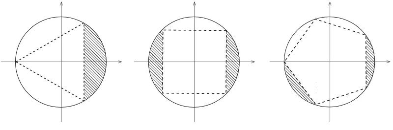
Fig. 1. {t}-Avoiding set fort= −12, 0 and cos25π.
10 Single Forbidden Inner Product
An interesting case to consider is when |X| =1, motivated by the fact that 1/α{t}(n)is
a lower bound on the measurable chromatic number of Rnfor anyt∈(−1,1)and this freedom of choosingtmay lead to better bounds.
Let us restrict ourselves to the special case when n=3 (that is, we look at the two-dimensional sphere). For a range oft∈[−1,cos2π5 ], the best construction that we could find consists of one or two spherical caps as follows. Givent, lethbe the maximum
height of an open spherical cap that is {t}-avoiding. A simple calculation shows that
h=1−√(t+1)/2. Ift≤ −1/2, then we just take a single capC of heighth, which gives thatα{t}(3)≥h/2 then. When −1/2<t≤0, we can add another cap C whose center is
opposite to that ofC. Whentreaches 0, the caps C andC have the same height (and
we get the two-cap construction from Kalai’s conjecture). When 0<t≤25π, we can form a
{t}-avoiding set by taking two caps of the same heighth. (Note that the last construction cannot be optimal for t>25π, as then the two caps can be arranged, so that a set of positive measure can be added; see the third picture of Figure1.)
Calculations show that the above construction gives the following lower bound
(whereh=1−√(t+1)/2):
α{t}(3)≥ ⎧ ⎪ ⎪ ⎪ ⎪ ⎨ ⎪ ⎪ ⎪ ⎪ ⎩
h
2, −1≤t≤ − 1 2,
h+t−ht, −1
2≤t≤0,
h, 0≤t≤cos2π 5 .
(17)
at University of Warwick on January 28, 2016
http://imrn.oxfordjournals.org/
We conjecture that the bounds in (17) are all equalities. In particular, our
con-jecture states that, for t≤ −1/2, we can strengthen Levy’s isodiametric inequality by forbidding a single inner producttinstead of the whole interval [−1,t].
As in Section 6, one can write an infinite linear program that gives an
upper bound on α{t}(3). Although our numerical experiments indicate that the upper
bound given by the LP exceeds the lower bound in (17) by at most 0.062 for all
−1≤t≤0.3, we were not able to determine the exact value of α{t}(3) for any single
t∈(−1,cos25π].
Acknowledgements
Both authors acknowledge Anusch Taraz and his research group for their hospitality during the summer of 2013. The first author thanks his thesis advisor Frank Vallentin for careful proofread-ing, and for pointing out the Witsenhausen problem [19] to him.
Funding
This work was supported by the European Research Council (GA 320924-ProGeoCom to E.D., GA 306493-EC to O.P.); the Netherlands Organisation for Scientific Research (639.032.917 to E.D.); the Lady Davis Fellowship Trust (to E.D.); and the Engineering and Physical Sciences Research Council (EP/K012045/1 to O.P.). Funding to pay the Open Access publication charges for this arti-cle was provided by EPSRC.
References
[1] Bachoc, C., E. DeCorte, F. M. de Oliveira Filho, and F. Vallentin. “Spectral bounds for the inde-pendence ratio and the chromatic number of an operator.”Israel Journal of Mathematics 202, no. 1 (2014): 227–54.
[2] Bachoc, C., G. Nebe, F. M. de Oliveira Filho, and F. Vallentin. “Lower bounds for measurable chromatic numbers.”Geometric and Functional Analysis19, no. 3 (2009): 645–61.
[3] Bachoc, C., A. Passuello, and A. Thiery. “The density of sets avoiding distance 1 in Euclidean space.”Discrete and Computational Geometry53, no. 4 (2015): 783–808.
[4] Dai, F. and Y. Xu. Approximation Theory and Harmonic Analysis on Spheres and Balls. Springer Monographs in Mathematics. Berlin: Springer, 2013.
[5] de Oliveira Filho, F. M. “New bounds for geometric packing and coloring via harmonic anal-ysis and optimization.” PhD Thesis, CWI, Amsterdam, 2009.
[6] Deitmar, A. and S. Echterhoff. Principles of Harmonic Analysis. Berlin: Universitext. Springer, 2009.
[7] Delsarte, P. “An algebraic approach to the association schemes of coding theory.” PhD Thesis, Universit ´e Catholique de Louvain, 1973.
[8] Delsarte, P., J. M. Goethals, and J. J. Seidel. “Spherical codes and designs.” Geometriae Dedicata6, no. 3 (1977): 363–88.
at University of Warwick on January 28, 2016
http://imrn.oxfordjournals.org/
[9] Folland, G. B. Real Analysis: Modern Techniques and Their Applications, 2nd edn. New York, United States of America: John Wiley & Sons Inc, 1999.
[10] Frankl, P. and R. M. Wilson. “Intersection theorems with geometric consequences.” Combinatorica1, no. 4 (1981): 357–68.
[11] Kalai, G. How large can a spherical set without two orthogonal vectors be? Combinatorics and more (weblog), 2009.
[12] Kalikow, S. and R. McCutcheon. An Outline of Ergodic Theory. Cambridge Studies in Advanced Mathematics 122, Cambridge, UK: Cambridge University Press, 2010.
[13] Larman, D. G. and C. A. Rogers. “The realization of distances within sets in Euclidean space.” Mathematika19, no. 1 (1972): 1–24.
[14] Levy, P.Probl `emes Concrets D’analyse Functionelle. Paris: Gauthier Villars, 1951.
[15] Raigorodskii, A. M. “On a bound in Borsuk’s problem.”Russian Mathematical Surveys54, no. 2 (1999): 453–4.
[16] Raigorodskii, A. M. “On the chromatic numbers of spheres inRn.”Combinatorica32, no. 1
(2000): 111–23.
[17] Schoenberg, I. J. “Metric spaces and positive definite functions.” Transactions of the
American Mathematical Society44, no. 3 (1938): 522–36.
[18] Szeg ¨o, G.Orthogonal Polynomials. Providence, RI: American Mathematical Society, 1992. [19] Witsenhausen, H. S. “Spherical sets without orthogonal point pairs.” American
Mathematical Monthly, no. 10 (1974): 1101–2.
at University of Warwick on January 28, 2016
http://imrn.oxfordjournals.org/