Data polygamy : the many many relationships among urban spatio temporal data sets

warwick.ac.uk/lib-publications

Original citation:

Chirigati, F., Doraiswamy, H., Damoulas, Theodoros and Freire, J. (2016) Data polygamy : the

many-many relationships among urban spatio-temporal data sets. In: ACM SIGMOD

International Conference on Management of Data, (SIGMOD 2016), San Francisco, 26 Jun -

01 Jul 2016. Published in: Proceedings of the 2016 ACM SIGMOD International Conference

on Management of Data, (SIGMOD 2016) pp. 1011-1025.

Permanent WRAP URL:

http://wrap.warwick.ac.uk/

Copyright and reuse:

The Warwick Research Archive Portal (WRAP) makes this work by researchers of the

University of Warwick available open access under the following conditions. Copyright ©

and all moral rights to the version of the paper presented here belong to the individual

author(s) and/or other copyright owners. To the extent reasonable and practicable the

material made available in WRAP has been checked for eligibility before being made

available.

Copies of full items can be used for personal research or study, educational, or not-for profit

purposes without prior permission or charge. Provided that the authors, title and full

bibliographic details are credited, a hyperlink and/or URL is given for the original metadata

page and the content is not changed in any way.

Publisher’s statement:

"© ACM, 2016. This is the author's version of the work. It is posted here by permission of

ACM for your personal use. Not for redistribution. The definitive version was published in

Proceedings of the 2016 ACM SIGMOD International Conference on Management of Data,

(SIGMOD 2016) pp. 1011-1025

http://doi.acm.org/10.1145/2882903.2915245

"

A note on versions:

The version presented here may differ from the published version or, version of record, if

you wish to cite this item you are advised to consult the publisher’s version. Please see the

‘permanent WRAP url’ above for details on accessing the published version and note that

access may require a subscription.

Data Polygamy: The Many-Many Relationships among

Urban Spatio-Temporal Data Sets

Fernando Chirigati

Harish Doraiswamy

Theodoros Damoulas

Juliana Freire

∗_{New York University} ?_{University of Warwick} †_{Alan Turing Institute}

{fchirigati,harishd,juliana.freire}@nyu.edu

[email protected]

ABSTRACT

The increasing ability to collect data from urban environments, coupled with a push towards openness by governments, has re-sulted in the availability of numerous spatio-temporal data sets cov-ering diverse aspects of a city. Discovcov-ering relationships between these data sets can produce new insights by enabling domain ex-perts to not only test but also generate hypotheses. However, dis-covering these relationships is difficult. First, a relationship be-tween two data sets may occur only at certain locations and/or time periods. Second, the sheer number and size of the data sets, coupled with the diverse spatial and temporal scales at which the data is available, presents computational challenges on all fronts, from indexing and querying to analyzing them. Finally, it is non-trivial to differentiate between meaningful and spurious relation-ships. To address these challenges, we proposeData Polygamy, a scalable topology-based framework that allows users to query for statistically significant relationships between spatio-temporal data sets. We have performed an experimental evaluation using over 300 spatial-temporal urban data sets which shows that our approach is scalable and effective at identifying interesting relationships.

1.

INTRODUCTION

Urban environments are the loci of economic activity and inno-vation. At the same time, most cities face huge challenges around transportation, resource consumption, housing affordability, and in-adequate or aging infrastructure. The growing volumes of urban data being collected and made available [3, 19, 26, 27, 32] open up new opportunities for city governments and social scientists to en-gage in data-driven science to better understand cities, make them more efficient, and improve the lives of their residents.

Urban data is unique in that it captures the behavior of the diff er-ent componer-ents of a city over space and time: its citizens, existing infrastructure (physical and policies), and the environment [20]. The availability of these data makes it possible to not only better understand the individual components but also obtain insights into how they interact. When an expert finds anunexpectedpattern or feature in a data set, other related data may help explain why and under which conditions the pattern occurs. Consider the top plot in

Permission to make digital or hard copies of all or part of this work for personal or classroom use is granted without fee provided that copies are not made or distributed for profit or commercial advantage and that copies bear this notice and the full citation on the first page. To copy otherwise, to republish, to post on servers or to redistribute to lists, requires prior specific permission and/or a fee.

Copyright 20XX ACM X-XXXXX-XX-X/XX/XX ...$15.00.

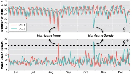
Figure 1: Variation of the number of taxi trips in NYC and its relationship with wind speed.

Figure 1, which shows the number of daily taxi trips in New York City (NYC) during 2011 and 2012. While the distribution of trips over time is very similar for the two years, we observe two large drops: one in August 2011 and another in October 2012. A natural question is what might have caused these drastic reductions. By ex-amining wind speed data (bottom plot in Figure 1), we discover that these drops occur on days with unusually high wind speeds; here, the high wind speeds were due to hurricanes Irene and Sandy. This suggests a new hypothesis to be further investigated: high wind speed leads to significant reduction in the number of taxi trips.

Besides enablinghypothesis generation, studying relationships among data sets can also help withhypothesis testing. For instance, the difficulty in finding taxis when it is raining is a notorious prob-lem in Manhattan. One long-standing hypothesis to explain this behavior is that taxi drivers set a daily income goal, and since there is higher demand on rainy days, they reach their goal faster and stop working earlier. Testing for the presence of such a relationship be-tween data sets—in this case, NYC taxi data and weather data—can help experts at the NYC Taxi and Limousine Commission (TLC) frame appropriate policies to counter identified problems.

Relationship Discovery. In this paper, we define and take a first step towards addressing the problem of discovering potential rela-tionshipsbetween spatio-temporal data sets. We aim toguideusers in the data analysis and exploration process by allowing them to poserelationship queries:

Find all data sets related to a given data setD.

Also, there is a large number of urban data sets. NYC alone has published over 1,300 data sets in the past two years [27], and this is just a small fraction of the data collected by the city. Since a data set can be related to zero or more data sets through multiple attributes, there is a combinatorially large number of possible relationships.

This problem is compounded by the fact that these data sets con-tain both spatial and temporal attributes at different resolutions. For example, values for the weather attributes are collected at hourly in-tervals (temporal resolution) for the whole city (spatial resolution). In contrast, NYC taxi trips are associated with GPS coordinates with time precision in seconds. Other data sets use spatial reso-lutions at the level of neighborhoods or zip codes, and temporal resolutions as daily, weekly, and monthly intervals. Since relation-ships can materialize at any of these resolutions, they should be evaluated at multiple resolutions.

The data complexity coupled with the sheer number of available data sets and the combinatorially large number of possible relation-ships make it hard for domain experts to comprehend the informa-tion and the insights it can potentially offer. Of the several thousand possible relationships between pairs of attributes in different data sets, only a small fraction is actually informative. Unless known a priori, looking for meaningful relationships between these data sets is like, as the cliché goes, “finding a needle in a haystack”.

Another challenge in identifying a possible relationship lies in defining the conditions implicating such a relationship. For exam-ple, consider the wind speed data and the NYC taxi trip data de-picted in Figure 1. There is no apparent relation between the two data sets during the normal course of time: it is only when the wind speed is abnormally high (in that case, due to hurricanes), that we can see a connection with taxi trips. This is a common pattern ob-served across urban data sets, where relationships become visible only atspatio-temporal regions(locations in space and time) that behave differently compared to the regions’ neighborhood.

Standard techniques, such as Pearson correlation coefficient [7] or dynamic time warping [21], do not capture these relationships because they ignore the spatio-temporal dependencies inherent in the data and operate globally over the entire data (see Section 6.4). Therefore, we need a method that captures the variation of the data over space and time at different and arbitrary resolutions.

Our Approach.To address these challenges, we propose theData Polygamyframework. We introduce the notion oftopology-based relationships, where two data sets are related if there is a rela-tionship between thesalient featuresof the data. A salient fea-ture corresponds to a spatio-temporal region that exhibits an un-usual behavior with respect to its neighborhood. To efficiently iden-tify salient features, we use and extend techniques from compu-tational topology. Topology-based techniques are naturally suited for studying properties of data involving spatial and geometric do-mains (e.g., see [11, 28, 38]). To give some intuition for why and how we apply topology, suppose we model a time step in an urban data set as a terrain, where the height of each point of the terrain represents the data value at that spatial location. In this case, the variation over space is captured by the peaks and valleys of this ter-rain. This can be extended to include time by modeling the data as a high dimensional terrain. The salient features, which as mentioned earlier correspond to spatio-temporal regions behaving differently from their neighborhood, are inherently represented as tall peaks and deep valleys. Topological methods provideefficient algorithms to represent and compute such features. In addition, they can iden-tify features that have anarbitrary spatial structureandstraddle multiple time intervals; they are alsogeneric, in the sense that they work on data having different dimensions and resolutions without requiring any modification.

Given two data sets, to determine whether they are related, we assess how similar their corresponding terrains are, i.e., the simi-larities in the spatio-temporal variation patterns of the data sets. In theData Polygamyframework, this is accomplished in three steps: 1. Data Set Transformation. Each attribute of the two data sets is transformed into ascalar function. A scalar function provides a mathematical representation of the terrain corresponding to a particular attribute of a data set.

2. Feature Identification.A topological data structure is computed for every scalar function, which provides an abstract representa-tion of the peaks and valleys of the scalar funcrepresenta-tion. This struc-ture is used as anindex to efficiently identify salient featuresin the data, which are defined based on thresholds that capture the extent of normal behavior of the scalar function. We develop a new method based on the notion oftopological persistence[8] to automatically compute these thresholds.

3. Relationship Evaluation.Possible relationships are then identi-fied based on feature similarity. Our framework filters out re-lationships that arenot statistically significant. Since existing Monte Carlo methods assume independence across samples, we develop restricted Monte Carlo permutation tests that respect data dependencies due to spatial and temporal proximity. Users can then pose relationship queries over the resulting ships. Hypothesis generation is supported by querying for relation-ships among all data sets, while a given hypothesis can be tested by querying for relationships between the data sets involved in the hypothesis. Sections 2, 3, and 4 provide the formal definitions and describe the algorithms used in these stages. The end-to-endData Polygamyframework is presented in Section 5.

Because we consider a large number of urban data sets, each containing many attributes, we need to compute thousands of scalar functions and derive millions of relationships. However, both salient feature identification and relationship querying are embarrassingly parallel operations. In Section 5.4, we briefly describe a map-reduce implementation of theData Polygamyframework.

We demonstrate the efficiency and robustness of our framework in Section 6 through an experimental evaluation using over 300 urban data sets of varying spatio-temporal resolutions. We also present use cases demonstrating its effectiveness at identifying in-formative relationships.

Note that our goal is to support users in the data exploration pro-cess by helping them discover data sets that may be relevant for their task—similar to a search engine that returns a set of poten-tially relevant documents for a given keyword query. Users can then use the identified relationships for further analysis, such as testing for spurious relationships, testing for causality (e.g., to sup-port a hypothesis), and generating new hypotheses.

Contributions.We define and propose a topology-based approach to the problem of identifying relationships across a large number of spatio-temporal data sets. Our main contributions are:

• We introduce the notion oftopology-based relationshipsto de-termine whether data sets are related through salient features.

• We develop ascalable frameworkthat identifies salient features based on the topology of the data, and a topology-based index that provides anoutput-sensitivestrategy to compute these fea-tures: the time taken is linear in the size of the output. We also propose analgorithm that automatically determines feature thresholds in a data-driven fashion.

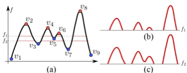
Figure 2: (a) A sample 1D scalar function. The labeled points form the set of maxima (red) and minima (blue). (b) The super-level set at f1 consists of four components. (c) The super-level

set atf2consists of three components.

• We describe a scalable, map-reduce implementation of theData Polygamyframework.

• We perform an extensive experimental evaluation, using real and synthetic data, which shows that our framework is robust, effi -cient, and effective.

2.

TOPOLOGY-BASED RELATIONSHIPS

In this section, we provide the required mathematical background and define the terms used in this paper, which are based on concepts from computational topology. We refer the reader to the following textbooks [13, 24] for a comprehensive discussion on these topics. We start by formally defining the concept of a topological feature and topology-based relationships. Then, we propose two measures to evaluate these relationships.

2.1

Topological Features

To discover relationships between two data sets, we first identify the set of topological features of thescalar functionsthat represent the data sets.

Scalar Functions.LetDbe a data set, andAan attribute ofD. To

identify the set of features with respect to the attributeA, we first represent the attribute as atime-varying scalar function.

Definition 1. Ascalar function f:_S→_Rmaps points on a spa-tial domainSonto a real value.

Definition 2. Atime-varying scalar function f: [S×T]→Rmaps

points on a spatial domain across time onto a real value.

The spatial resolution of the data setDdetermines the structure

of the spatial domain_S. For example, the NYC weather data set provides information on different climate attributes, such as tem-perature, precipitation, and wind speed. The values of these at-tributes correspond to an hourly time period for the entire city, i.e., all the values correspond to the same spatial point. In this case, the domainS×Tof the time-varying scalar function is a simple time

series, i.e., a 1D function (0D in space and 1D in time). Figure 2(a) and the two time series shown in Figure 1 are examples of 1D scalar functions. On the other hand, the NYC taxi data consists of a set of taxi trips, each containing the GPS coordinates for pick-up and drop-offlocations. From these data, we can obtain a distribution of taxi trips over space and time by partitioning NYC into a set of polygons (e.g., neighborhoods) and counting the trips that start (or end) in each polygon at different time steps. This is adensity function, where the spatial domain is 2D, and thus the time-varying scalar function is 3D (2D in space and 1D in time). Figure 3 shows the density function at two different spatial resolutions for one time step (i.e., one hour time period). The different scalar functions that can be used to represent a data set are discussed in Section 5.1.

Irrespective of the temporal resolution, time always contributes to one dimension in the time-varying scalar function. Unless oth-erwise noted, we use the termscalar functionto refer to a time-varying scalar function corresponding to a (data set, attribute) pair.

Topological Features. Interesting features of a scalar function f

are captured by thecritical pointsof f.

Figure 3: One time step (2D slice) of the 3D function repre-senting the density of taxi trips in NYC at different resolutions. Dark and light regions correspond to high and low trip density, respectively. (a) NYC is represented using a high-resolution grid and the density is provided for each cell of this grid. (b) A lower resolution, at the level of neighborhood, is used.

Definition 3. Given a smooth function f, thecritical pointsoff

are the points where the gradient becomes zero, i.e.,∇f=0. We assume that the scalar functionfis a Morse function [24]. A Morse function has the property that (i) no two critical points have the same function value; and (ii) there are no degenerate critical points (i.e., ∇2f ,0). Any continuous function f can be made

Morse via a simulated perturbation offby an infinitesimally small value such that no two points have the same function value [12]. We provide a detailed discussion on Morse functions in Appendix B.1. We are interested in two particular types of critical points, maxi-mumandminimum, collectively known asextrema. Given a Morse function, maximum and minimum points are defined as follows:

Definition 4. A pointxis amaximumiff(x)>f(x0),∀x0∈N(x), whereN(x) defines the local neighborhood ofx. Similarly,xis a

minimumiff(x)<f(x0),∀x0∈N(x).

The red and blue points in Figure 2(a) correspond to the set of maxima and minima, respectively. We use the neighborhood of critical points of a function to represent the topological features of the data. The neighborhoods of the maxima and minima of fare captured by thesuper-levelandsub-level setsof f, respectively.

Definition 5. Given a scalar function f, thesuper-level setat a real valueθis defined as f−1([θ,∞)), i.e., the pre-image of the interval [θ,∞). Thesub-level setatθis defined as f−1((−∞,θ]).

In other words, the super-level set at a real valueθis the set of all points on the domain of f having function value greater than or equal toθ. For example, the super-level set of the function in Figure 2(a) at function value f1 consists of 4 components

(Fig-ure 2(b)), while the super-level set at f2consists of 3 components

(Figure 2(c)). Similarly, the sub-level set atθis the set of all points in the domain offhaving function value less than or equal toθ.

We define two types of features—positive and negative—using super-level and sub-level sets, respectively.

Definition 6. Given a feature threshold θ+, the set of positive featuresis defined as the super-level set f−1([θ+,∞)).

Definition 7. Given an feature thresholdθ−_{, the set ofnegative}

featuresis defined as the sub-level setf−1((−∞,θ−]).

Feature Representation.The spatial domainSofDis represented

as a set of regions{s1,s2,...,sn}that partition the spatial extent of D. Each regionsicorresponds to a polygon defined by the

Definition 8. Aspatio-temporal pointis represented by a (spa-tial region, time interval) pair.

Topological features of fcorrespond to a set of spatio-temporal points over the domain of f. Intuitively, they represent spatio-temporal points where attributeAof data setDdeviates from its

normal behavior, and capture the variation ofAover both space and time. Here, the thresholdsθ+andθ−define the extent of nor-mal behavior ofA. Salient features of the function can be identified by appropriately setting the values of these thresholds. For exam-ple, using the indicated values ofθ+andθ−in Figure 1, features corresponding to the hurricanes are obtained. We describe an algo-rithm to identify the appropriate values forθ+andθ−in Section 3.3.

2.2

Feature Relatedness

Consider two scalar functions: f1(D1,A1) corresponding to

at-tributeA1of data setD1, andf2(D2,B1) corresponding to attribute

B1ofD2. Without loss of generality, we assume that the two

func-tions have the same spatial and temporal resolution. LetΣ1andΣ2

be the set of features off1and f2, respectively. LetΣ = Σ1TΣ2be

the set of all spatio-temporal points that are features in bothf1and

f2. The possible relationships between two functions are defined

based on the relationship between their features.

Definition 9. Two functions f1 and f2 arefeature-related at a

spatio-temporal pointx=(s,t) ifx∈Σ.

At points not inΣ, the two functions are not feature-related. Let

Σ+

i ⊂Σibe a set such that∀x∈Σ+i,xis a positive feature. Similarly,

letΣ−_i ⊂Σibe the set of negative features.

Definition 10. f1andf2arepositively relatedat a spatio-temporal

pointx∈Σif (x∈Σ+₁andx∈Σ+₂) or (x∈Σ−₁ andx∈Σ−₂).

Definition 11. f1andf2arenegatively relatedat a spatio-temporal

pointx∈Σif (x∈Σ+

1andx∈Σ

−

2) or (x∈Σ

−

1 andx∈Σ+2).

For instance, consider the features from Figure 1 correspond-ing to the indicated thresholds. At the spatio-temporal point corre-sponding to hurricane Sandy, there is a negative feature in the taxi density function and a positive feature in the wind speed function. The functions are therefore negatively related at that point.

2.3

Relationship Score and Strength

To assess the relationship between a given pair of functions, we define the following two measures.

Relationship Scoreτ. We are interested in evaluating the overall nature of the relationship between two functions, i.e., whether it is always positive, always negative, or somewhere in between. To do so, we define therelationship scoreτbetween two functions

f1(D1,A1) andf2(D2,B1). LetΣ1andΣ2denote the set of features

of f1and f2, respectively. As defined earlier, the setΣ = Σ1TΣ2

denotes the feature-relations between the two functions. Let #pand #nbe number of positive and negative feature relations inΣ. The relationship score is defined as

τ=#p−#n

|Σ| (1)

A value ofτcloser to+1 indicates that the two functions are posi-tively related, while a value closer to−1 indicates that the functions are negatively related.

Relationship Strengthρ.This measure is used to capture how fre-quently features in two functions are related: the more frefre-quently the features are related, the stronger the relationship is. We model the set of features as binary classifiers. Consider any spatio-temporal pointx∈Σ1. Ifxis also present inΣ, it is considered as a true

pos-itive. A pointxis a false positive whenx∈Σ1andx<Σ. Similarly,

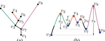
Figure 4: (a) Join tree of the function shown in Figure 2. The edges are colored based on the descending path traversed from the corresponding maxima illustrated in (b).πidenotes the per-sistence of maximumvi.

xis false negative whenx<Σ1andx∈Σ. We then use the F1 score

to measure the relationship strength as

ρ=F1(f1,f2)=2×

precision×recall

precision+recall (2)

Note that precisiongives a measure of how often features in f1

are related with features in f2, andrecallgives a measure of how

often features in f2are related with features in f1. Thus, a value

of ρcloser to 1 indicates a strong relationship between the two functions, since a feature in one function almost always indicates a feature in the other function as well. Similarly, a value ofρclose to zero indicates a weak relationship.

3.

MERGE TREE INDEX

We use a topological data structure called merge treeto effi -ciently identify salient features corresponding to a scalar function. In what follows, we give an overview of merge trees and introduce a new algorithm to compute the features thresholdsθ+andθ−, a crucial step in this process.

3.1

Index Creation

Recall that a super-level set (or sub-level set) of a scalar function

f at a given function value consists of multiple connected com-ponents. Therefore, decreasing or increasing the function values changes the topology, i.e., the number of connected components. A

merge treetracks the evolution of super-level sets or sub-level sets of fwith changing function value. Formally, there are two types of merge trees.

Definition 12. Thejoin treeof f tracks the connected compo-nents of the super-level sets of fwith decreasing function value.

Definition 13. Thesplit treeof f tracks the connected compo-nents of the sub-level sets of fwith increasing function value.

Consider the 1D function shown in Figure 2(a). At the highest function value, a single super-level set component is created atv8.

As we decrease the function value, the number of components re-main at one until the function value is equal to that of thev2. As

we keep decreasing the function value, two more components are created atv4followed byv6(Figure 2(b)). However, when the

func-tion value reachesv5, the components created atv4 andv6 merge

into one component, reducing the number of components from 4 to 3 (Figure 2(c)). We stop this process when the function value goes belowv1(the global minimum). At this point, there is a single

super-level set component composed of the entire domain. The join tree tracks this evolution as a graph. Figure 4(a) shows the join tree of the 1D function from Figure 2(a). The nodes of the graph cor-respond to critical points where the number of components change, while an edge represents the connected super-level set component between its end points. For example, the edge (v2,v3) corresponds

the root node of a split tree corresponds to the global maximum and its non-root leaf nodes correspond to the set of minima of f. In order to compute merge trees, we first have to obtain a discrete representation of a scalar function, which we describe next.

Scalar Function Representation.Consider the spatial domain of a data setDconsisting of regions{s1,s2,...,sn}. Let the

tempo-ral domain ofDconsist ofmtime steps{t1,t2,...,tm}. We create a

graphG=(V,E) to represent the spatio-temporal domain ofDas

follows. Vertexvx,z∈Vrepresents the spatio-temporal point

cor-responding to regionsxat timetz. Thus,|V|=n×m. The edges

E=ESSETare divided into two categories:

• spatial edges:ES ={(vx,z,vy,z)|sxadjacent tosy,∀z∈[1,m]} • temporal edges:ET={(vx,z,vx,z+1),∀x∈[1,n],z∈[1,m)}

Edges inES connect adjacent regions of the space for each time

step, and edges inETconnect a region across adjacent time steps.

We use a piecewise linear (PL) function defined onGto represent the scalar function f: the function is defined on the vertices of

G and linearly interpolated within each edge. The graph allows a single representation to be used irrespective of the dimension of the spatio-temporal domain, thus supporting different resolutions and dimensions of the data.

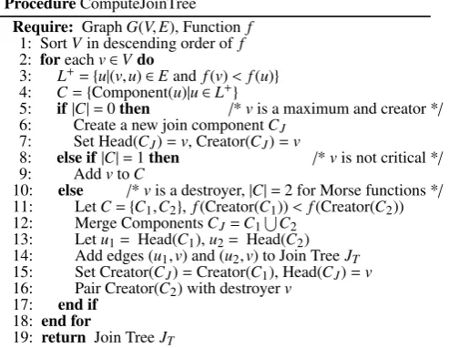
Merge Tree Computation.The merge tree of a PL function can be efficiently computed inO(NlogN+Mα(M)) time using the union-find data structure, whereNandMare the number of vertices and edges, respectively, inG. Since the spatial domains considered in this work correspond to cities, the graphGrepresenting these domains is planar. Thus,M=O(N). The algorithm to compute join trees is given in Procedure ComputeJoinTree (for more details, see Appendix B.2). The split tree is computed analogously by using the functionf0=−fin this algorithm.

3.2

Querying Features

We use the join and split trees as indices to efficiently compute the set of features, i.e., the super-level sets and sub-level sets, re-spectively. Letθbe the feature threshold. The algorithm to compute the super-level setf−1([θ,∞)) using the join treeJTis as follows:

1. Identify the setV+={v|vis a maximum and f(v)≥θ}. This is accomplished by going over the non-root leaf nodes ofJT.

2. SetΣ+=∅. 3. WhileV+,∅

(a) RemovevfromV+and add toΣ+.

(b) LetL−={u|f(u)≤f(v) anduis adjacent tov}. (c) Addu∈L−toV+ifθ≤f(u).

4. The setΣ+contains the vertices ofGthat belong to the super-level set atθ.

The algorithm performs a descending path traversal of adjacent ver-tices from the set of valid maxima (having function value greater thanθ) until the required threshold is reached. The colored regions in Figure 4(b) indicate the descending paths followed by the algo-rithm starting from the different maxima of the function shown in Figure 2(a). This is analogous to traversing down the edges of the join tree. The sub-level set atθis computed similarly, through an ascending path traversal starting from the minima of the function.

Time Complexity.Since the vertices ofGare sorted when comput-ing the join (or split) tree, the critical points of the function are also stored in sorted order. Thus, the number of comparisons required to identifyV+(orV−) is|V+|(or|V−|). Each descending (or ascend-ing) path traversal stops as soon as it reaches a vertexuthat is not a feature. Thus, the number of vertices touched during querying is

O(Σ+) (orO(Σ−)). In other words, given the join and split trees, feature identification for a given threshold isoutput-sensitive.

ProcedureComputeJoinTree

Require: GraphG(V,E), Function f

1: SortVin descending order off

2: foreachv∈Vdo

3: L+={u|(v,u)∈Eand f(v)<f(u)}

4: C={Component(u)|u∈L+}

5: if|C|=0then /*vis a maximum and creator */ 6: Create a new join componentCJ

7: Set Head(CJ)=v, Creator(CJ)=v

8: else if|C|=1then /*vis not critical */ 9: AddvtoC

10: else /*vis a destroyer,|C|=2 for Morse functions */ 11: LetC={C1,C2}, f(Creator(C1))<f(Creator(C2))

12: Merge ComponentsCJ=C1SC2

13: Letu1= Head(C1),u2= Head(C2)

14: Add edges (u1,v) and (u2,v) to Join TreeJT

15: Set Creator(CJ)=Creator(C1), Head(CJ)=v

16: Pair Creator(C2) with destroyerv

17: end if

18: end for

19: return Join TreeJT

3.3

Feature Threshold Computation

Intuitively, our goal is to classify topological features not adher-ing to normal behavior assalient features. We are also interested in identifyingextreme features, which correspond to outliers among salient features. For instance, the extremely high wind speeds dur-ing a hurricane correspond to extreme features

While users with domain knowledge can provide thresholds for computing features, this might not be feasible over all data sets. Thus, we devise a data-driven approach to identify the required thresholds,θ+andθ−. Our approach is inspired by thepersistence diagram [8], which is commonly used in scientific visualization applications to visually identify meaningful thresholds [11]. How-ever, instead of relying on users to visually select thresholds, we develop an algorithm to automatically identify them.

Topological Persistence. Consider a sweep of the function f in decreasing order of function value. As mentioned earlier, the topol-ogy of the super-level set changes at critical points during this sweep. In particular, at a critical point, either a new super-level set nent is created (maximum) or an existing super-level set compo-nent is destroyed. A critical point is acreatorif a new component is created, and adestroyerotherwise. Again, consider the exam-ple in Figure 4. At critical pointv5, the components created atv4

andv6 are merged into one. In this case, the component created

last, atv6, is considered to be destroyed atv5. Similarly, one can

pair up each creatorc1uniquely with a destroyerd1that destroys

the topology created atc1. Note that this pairing can be

accom-plished while computing the merge tree itself (Line 16 in Proce-dure ComputeJoinTree). Thepersistence valueofc1andd1is

de-fined as|f(d1)−f(c1)|, which indicates the lifetime of the feature

created atc1. Figure 4(b) illustrates the persistence values of the

different critical points (asπi) together with the creator-destroyer

pairs. Intuitively, the persistence of a maximum (minimum) is equal to the height (depth) of the corresponding peak (valley).

(maxi-mum) with a higher persistence value is considered important since the sub- (or super-) level set component created at that extremum has a longer lifetime. Our goal is to select a thresholdθ−such that all the high persistence minima are identified as salient. To do this automatically, we performk-means clustering withk=2 and use the highest value over all minima in the high persistence cluster as the thresholdθ−. This ensures that all the high-persistence minima will have function value less than or equal toθ−, and will hence be identified as salient features. θ+is identified in a similar manner using the persistence of the set of maxima.

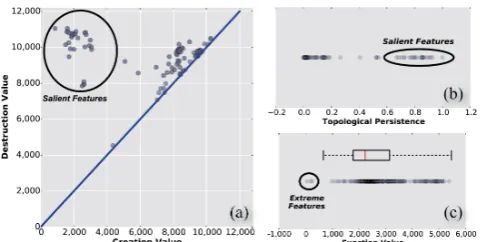
Thresholds for Extreme Features. Typically, a minimum (maxi-mum) corresponding to an extreme feature will have function value that is significantly smaller (larger) than those corresponding to salient features. For example, in Figure 5(c), the function value of minima corresponding to the extremely low number of taxi trips in NYC between 2009 and 2013 is significantly different from the function value of other minima (corresponding to salient features). In order to identify the appropriate thresholds, we first compute the minima (or maxima) across all time steps that correspond to salient features. Next, we identify the outlier threshold from this distribu-tion. We use the standard box plot thresholds, i.e.,Q1−1.5×IQR

for minima (Q3+1.5×IQRfor maxima), as the required

thresh-olds, whereQ1andQ3are the first and third quartile, andIQRis

the inter-quartile range. The box plot (and the corresponding out-lier threshold) for the extreme negative features corresponding to the taxi density function is illustrated in Figure 5(c).

Adjusting for Seasonal Variations. Processes in a city are typi-cally dependent on the time of year. For example, zero depth of snow during summer is normal, while this could indicate an impor-tant phenomena during the winter. Thus, it is imporimpor-tant to take into account seasonal variations when computing features. Depending on the temporal resolution, the time range of a data set is divided into smaller intervals, and the threshold for a given interval is com-puted based on the persistence of the extrema present in that inter-val. For example, we could use monthly or quarter-yearly intervals.

4.

RELATIONSHIP OPERATOR

In the previous sections, we discussed how relationships between functions are identified and measured. We now define the relation-ship operator,relation(D1,D2), used to compute the relationship

between data setsD1 andD2. LetD1be represented byn

func-tions{f1,f2,...,fn}, andD2bymfunctions{g1,g2,...,gm}. There

aren×mpossible relationships between the two data sets. Since many of these relationships could be due to random chance, the relationship operator returns the set of statistically significant rela-tionship pairs (fi,gj) together with their corresponding relationship

score and strength.

To assess the statistical significance of a potential relationship pair (fi,gj), we design Generalized Monte Carlo significance tests

[5, 15, 18]. LetΣ1andΣ2be the features corresponding to fiand

gj, respectively. The null and alternative hypothesis are:

H0: The two functionsfi,gjare independent in their featuresΣ1,Σ2.

H1: The two functions are dependent in their features.

We examine if we can reject the null hypothesis and acceptH1for

any pair of functions based on the identified features and their cor-responding relationship score. Thep-value from the Monte Carlo randomization test with test statisticx∗is given by:

p=P(X≤x∗|H0)=

PN

i I(xi≤x ∗₎

N as N→ ∞ (3)

where I(·) is the indicator function andNthe number of permuta-tions on the input. Given a significance levelα, thep-value is then used to define a statistically significant relationship as follows:

Figure 5: (a) The persistence of a minima in a persistence di-agram is the height above thex=yline. (b) A scatter plot of the persistence of the minima. (c) When considering only nega-tive features across all time intervals, note that function values corresponding to extreme features (e.g., during hurricanes) are outliers of the distribution.

Definition 14. The relationship between two functions fiandgj

is statistically significant ifp≤α.

Urban data sets have spatial and temporal dependencies (e.g., due to neighborhood and seasonal effects) that need to be accounted for when designing randomization tests. It is well-known in the statistics literature that, if we ignore these dependencies, a simple Monte Carlo procedure for assessing statistical significance would fail and lead to erroneous claims [5, 23]. To account for the spatio-temporal correlation, a plethora of Monte Carlo and Bootstrap tech-niques have been developed over the last decades ranging from the block-bootstrap [22] to general restricted Monte Carlo techniques [18, 23] such as the one we propose in this paper.

Restricted Monte Carlo Tests for Spatial Correlation. We de-velop restricted permutation tests that respect the degree of spatial correlation of our data sources. This is typically achieved by de-signing toroidal shifts, where a function f is wrapped around a two-dimensional torus by connecting the margins, or spatial ex-tents, of the data. Then, a linear mapm—that maps the torus onto a rotation of itself—will yield a new randomization that still respects any horizontal interactions [18, 23].

However, given the irregular structure of a city, which is an arbi-trary non-convex polygon, wrapping the spatial region over a torus is not straightforward. If we consider the spatial domain as a graph, a toroidal shift basically ensures that the adjacency of the non-boundary vertices are maintained. We make use of this observation to devise a toroidal shifting strategy that is applicable to arbitrary graphs. Given a graphGrepresenting the spatial domain, we define the mapmi:G→Gas follows. We start with a random mapping

mi(u)=v. The adjacent vertices ofuare then assigned the

ver-tices adjacent tovwhere applicable. This process is repeated in a breadth-first fashion. This process ensures that, in most cases, the distance between two vertices inGis the same as the distance between them inmi(G). Using the above mapping, the restricted

Monte Carlo test now becomes:

p=

P|m|

k I(τ(fi,gj)k≤τ(fi,gj)∗)

|m| (4)

whereτ(fi,gj)kis the relationship score between the two functions

fi,gjin toroidal shiftk, and|m|is the total number of toroidal shifts,

which affects the power of the statistical test (we use|m|=1,000).

correla-tions [18]. We then proceed similarly to Equation 4. Unless oth-erwise mentioned, a relationship implies a statistically significant relationship for the remainder of the paper.

5.

DATA POLYGAMY FRAMEWORK

In this section, we describe the data polygamy framework. We start by presenting thescalar functions that are derived from a given data set and how the framework handles different resolutions. Then, we discuss how the data is indexed and queries are evalu-ated. Finally, we briefly describe a map-reduce implementation of the framework.

5.1

Types of Scalar Function

Consider a data set_Dhaving attributes{K,S,T,A1,A2,...,Ak}.

LetKbe an optional unique identifier;S andT be the spatial and temporal attributes, respectively; andAi,1≤i≤kbe numerical

at-tributes. We are interested in identifying scalar functions that not only capture the activity of the objects represented by the data sets, but that also that capture the different properties corresponding to the attributes. For instance, when considering the taxi data, the number of taxis in different locations over time captures the activity of the taxis, while the attribute corresponding to the fare captures fare patterns over time and space. We therefore derive two types of scalar functions to representD: count functions andattribute

functions. Possible extensions to other types of scalar functions are discussed in Section 8.

Count Functions.Count functionsare used to capture the activity of the entity represented by the data set. More formally, consider a spatio-temporal point (s,t). LetΓbe the set of tuples inDsuch

thatS(r)=sand T(r)=t,∀r∈Γ. Here,S and T represent the spatial and temporal attributes of a tupler. We define two types of count functions:densityandunique. Thedensity functionassigns the value|Γ|to the spatio-temporal point (s,t). For example, the density function of the taxi data assigns the number of trips origi-nating atsduring the time periodtto the point (s,t). Theunique functionassigns a value equal to the number of unique identifiers ofΓto the spatio-temporal point. For instance, each tuple in the taxi data consists of an identifier corresponding to the medallion of the taxi. Thus, the number of unique medallions inΓis essentially the number of unique taxis that are present atsduring timet. Note that there is one unique function corresponding to each identifier attribute of the data set.

Attribute Functions.For a given attributeA, theattribute function

assigns the average value ofA(r) over all tuplesr∈Γto the cor-responding spatio-temporal point (s,t); the function represents the variation in the properties of a given attribute over space and time.

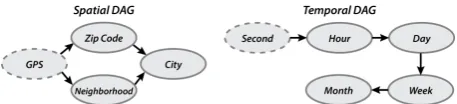
Handling Different Data Resolutions. It is important that our framework identifies relationships that occur at different resolu-tions. As illustrated in Figure 6, these resolutions are represented as a directed acyclic graph (DAG), where the edges are directed from a higher resolution to a compatible lower resolution. The compat-ibility indicates the ability to convert the data from a higher reso-lution to a coarser resoreso-lution. For example, GPS resoreso-lution can be transformed into all of the other resolutions. On the other hand, neighborhood and zip-code resolutions, being incompatible, can be converted only into the city resolution. To evaluate the relationship between two functions having different resolutions, we first trans-form both functions into the same compatible resolution, and then evaluate the two functions at this resolution.

5.2

Indexing and Feature Identification

Given a data setD, we first compute all possible scalar functions

(i.e., count and attribute functions) ofDthat cover every viable

Figure 6: Hierarchical relationship for spatio-temporal resolu-tions represented by DAGs. Resoluresolu-tions depicted using solid lines are used for evaluating relationships.

spatio-temporal resolution. For example, ifDis available at a

spa-tial resolution of GPS locations and temporal resolution of second, then each attribute can be aggregated into 3 spatial resolutions (i.e., zip code, neighborhood, and city) and 4 temporal resolutions (i.e., hour, day, week, and month), thus resulting in a total of 12 spatio-temporal resolutions for which the scalar functions are computed. The merge tree index is then built for each scalar function. This ensures that all resolutions are considered when executing a rela-tionship query. Recall that the computation of feature thresholds takes seasonal variations into account (Section 3.3). In particular, we use monthly and quarter-yearly intervals when the temporal res-olution is hourly and daily, respectively. Since thresholds are fixed for a given function, to speed up query evaluation, we pre-compute and store the features (salient and extreme).

5.3

Query Evaluation

LetD={_D1,...,_Dn} be the corpus of data sets that have been indexed. We support the general form of therelationship query:

Find relationships betweenD1andD2satisfyingclause

In this query, D₁ and D₂ are collections of data sets such that

D1⊆ DandD2⊆ D. IfD2=∅, it is assumed thatD2=D. When

a relationship query is issued, therelationoperator is applied to all

pairs (_Di,Dj) of data sets, such thatDi∈ D1,Dj∈ D2, andDi,Dj.

The operator uses the pcomputed set of features to assess the re-lationship between the data sets. Note that, when considering a pair of functions, the relationship between them is evaluated for all pos-sible resolutions starting with thehighest commonresolution. For example, if the spatial resolutions of two functions are neighbor-hood and zip code, then their relationship is evaluated at the city scale for different possible temporal resolutions. This evaluation is performed for both salient and extreme features.

Computing relationships at different resolutions is important as scalar functions may relate differently depending on how they are aggregated. For example, an hourly resolution might capture varia-tions within a day, but could miss significant variavaria-tions across dif-ferent days, which can be captured using a daily resolution (see Section 6.3 for an example).

The query returns related scalar function pairs that are statisti-cally significant, together with the resolutions for which the rela-tionships hold. The significance levelαis set at the commonly used value of 5% [15]. In theclausefor a query, optional condition

parameters can be specified to filter relationships satisfying a min-imum scoreτand/or strengthρ. Feature thresholds for computing salient and extreme features can also be optionally specified as part of theclauseif the user is familiar with any of the data sets. When

these thresholds are specified, features are first identified using the merge tree index before evaluating the relationship.

5.4

Implementation

Given a large number of data sets, such as the urban data sets with which we experimented (Section 6), thousands of scalar func-tions have to be computed, and the number of relafunc-tionships to be evaluated during querying is in the order of millions. However, the indexing and querying operations can be run independently for each scalar function and scalar function pair. To leverage the

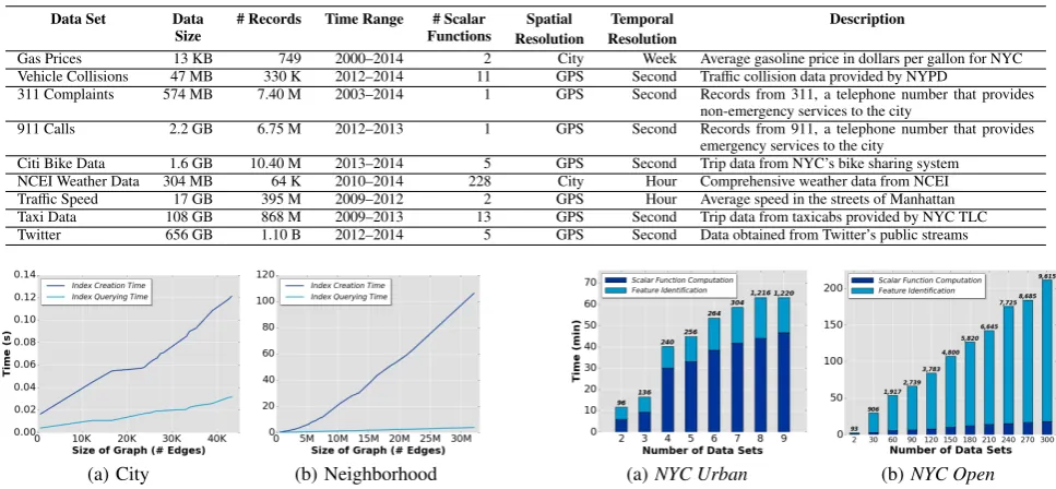
imple-Table 1: Properties of the data sets in theNYC Urbancollection.

Data Set Data

Size

# Records Time Range # Scalar Functions

Spatial Resolution

Temporal Resolution

Description

Gas Prices 13 KB 749 2000–2014 2 City Week Average gasoline price in dollars per gallon for NYC

Vehicle Collisions 47 MB 330 K 2012–2014 11 GPS Second Traffic collision data provided by NYPD

311 Complaints 574 MB 7.40 M 2003–2014 1 GPS Second Records from 311, a telephone number that provides

non-emergency services to the city

911 Calls 2.2 GB 6.75 M 2012–2013 1 GPS Second Records from 911, a telephone number that provides

emergency services to the city

Citi Bike Data 1.6 GB 10.40 M 2013–2014 5 GPS Second Trip data from NYC’s bike sharing system

NCEI Weather Data 304 MB 64 K 2010–2014 228 City Hour Comprehensive weather data from NCEI

Tra_ffic Speed 17 GB 395 M 2009–2012 2 GPS Hour Average speed in the streets of Manhattan

Taxi Data 108 GB 868 M 2009–2013 13 GPS Second Trip data from taxicabs provided by NYC TLC

Twitter 656 GB 1.10 B 2012–2014 5 GPS Second Data obtained from Twitter’s public streams

(a) City (b) Neighborhood

Figure 7: Merge tree index creation and feature querying time.

mented the framework usingmap-reduce. We use threemap-reduce

jobs: 1.Scalar Function Computationgenerates all possible scalar functions at different resolutions; 2.Feature Identificationcreates the merge tree indexes and identifies the set of features of the dif-ferent functions; and 3.Relationship Computationevaluates the re-lationships between the pairs of functions corresponding to a given query. Implementation details can be found in Appendix C and the released code.1

Space Overhead. The space required to store a scalar function for a given resolution is equal to the number of vertices in the graphGrepresenting the domain. For a resolution at the city level and hourly intervals, this corresponds to the number of time steps, which is approximately 35 KB (365×24 float values) per year. For higher spatial resolutions, the space required to store the function is approximatelyn×35 KB, wherenis the number of polygons used to partition the domain. For example, in NYC, for zip code and neighborhood resolutions,n≈300. Typically, the space over-head to store scalar functions over all resolutions is significantly less than the original data itself. As a point of reference, the 5 years of the raw taxi data takes up 108 GB of space. In contrast, the 13 possible scalar functions over 8 resolutions uses only 417 MB. The size of the merge tree index is proportional to the number of crit-ical points of the function. While the number of critcrit-ical points is bounded by the size of the input graph in the worst case, in practice it is significantly smaller. Similarly, even the number of features, while being bounded by the size of the input graph, is usually much smaller. For example, storing all features (salient and extreme) for the taxi data over all different resolutions takes only 8 MB.

6.

EXPERIMENTAL EVALUATION

We have performed an extensive evaluation to assess different aspects of theData Polygamyframework. We carried out a con-trolled experiment to quantitatively evaluate the correctness and ro-bustness of the relationship operator, and we also used real-world data sets to study efficiency and effectiveness characteristics. Ef-ficiency was measured to show the feasibility of computing

rela-1_{URL of the code is withheld due to the double blind requirement.}

(a)NYC Urban (b)NYC Open

Figure 8: Performance of feature indexing and identification.

tionships over a large number of data sets. Effectiveness was eval-uated in two different ways: to demonstrate that the framework is able to prune spurious relationships, thus reducing the exploration space presented to users, and to show that our approach uncovers

interesting, non-trivial relationships. We also analyzed the rela-tionships obtained from standard correlation techniques and discuss their shortcomings in identifying interesting relationships.

Experimental Setup. We used Apache Hadoop 2.2.0 and Java 1.7.0. Themap-reducejobs were executed on a cluster with 20 compute nodes, each node having an AMD Opteron(TM) Proces-sor 6272 (4x16 cores) running at 2.1GHz, and 256GB of RAM.

Data Sets.We used two collections of data sets in our experiments. The NYC Urbancollection consists of nine urban data sets ob-tained from different NYC agencies or gathered through publicly-available APIs. These data sets have been used by various domain experts (mostly in isolation) for different analyses (see, e.g., [6, 17]) and are thus useful to evaluate the effectiveness of our framework at identifying meaningful relationships. Table 1 describes these data sets and their properties. They vary in size from a few KBs to hun-dreds of GBs, and have different temporal and spatial resolutions.

The second collection, referred to asNYC Open, was primarily used to test the performance of our framework. It consists of 300 spatio-temporal data sets from NYC Open Data [27]. Even though most of these data sets are relatively small in size (less than 1 GB), the sheer number of data sets and the number of attributes they contain (on average, 8 attributes per data set) results in over 2.4 million possible relationships for a single resolution.

Each data set in these collections consists of a set of tuples hav-ing metadata about the spatial, temporal, and numerical attributes as well as keys. We use this metadata to perform an additional pre-processing step that selects data corresponding to these attributes and feeds it to the scalar function computation module.

6.1

Performance Evaluation

(a)NYC Urban (b)NYC Open

Figure 9: Query performance.

create the index and query for features for the Taxi data (using its density function), for both city (1D) and neighborhood (3D) resolu-tions. Here, we used a single node in the cluster. The plots indicate that the time for creating the merge tree and identifying features is almost linear in the size of the function (i.e., number of edges in the spatial domain graph). Note that the indexing time includes the creation of both join and split trees, and the querying time includes the computation of thresholds as well as the identification of neg-ative and positive features. Even for an input having more than 30 million edges, the operations took less than 2 minutes. This shows that our approach is scalable and able to handle large data sets.

The indexing component also performs well as the number of data sets increases. This is shown in Figure 8. The numbers on the bars indicate the total number of computations performed. Recall that scalar functions are computed for all attributes at all spatio-temporal resolutions. When usingNYC Urban(Figure 8(a)), the large increase in time when moving from 3 to 4 data sets was due to the 4thdata set, the Taxi data, which is not only large but also contains many attributes. It also has the highest resolution both in space and time, requiring each scalar function to be computed over all resolutions. There was also a significant increase in the number of computations when the Weather data set was introduced (the 8th data set): this data set has 228 numerical attributes. However, since it is relatively small compared to other data sets inNYC Urban, the running time was not significantly affected.

ForNYC Open(Figure 8(b)), the time taken to identify the fea-tures was significantly larger than that for computing the scalar functions. This behavior differs from what we observed forNYC Urbandue to two reasons: (1) the data sets in this collection are much smaller; (2) most of the 3D data sets inNYC Openare al-ready in zip code resolution, making it faster to compute the scalar functions; in contrast, tuples in the 3DNYC Urbandata sets are GPS points, which required additional computations to aggregate into the neighborhood and/or zip code resolutions. The total time taken to compute the indexes and features for all data sets inNYC UrbanandNYC Openwas about 1 hour and 4 hours, respectively.

Query Performance.To test the efficiency of the querying compo-nent, we executed a series of queries that identify the relationships between a fixed number of data sets. Figure 9 plots the relationship evaluation rate with increasing number of data sets. Using both collections,NYC UrbanandNYC Open, we were able to consis-tently evaluate relationships at a rate greater than 104relationships per minute. The evaluation rate stabilized once the number of rela-tionships increased above this number, e.g., with the addition of the Weather data (data set 8) in Figure 9(a). A total of 290 thousand relationships were evaluated when the query used all data sets from

NYC Urban; for theNYC Open, this number was 17.4 million. The constant rate, irrespective of the data set pairs, indicates that re-lationship evaluation is independent of size and resolution of the original data. This can be attributed to the abstraction of the data as functions. Note that over 90% of the querying time is spent on the statistical significance tests, which involve re-evaluating each

rela-(a)NYC Urban (b)NYC Open

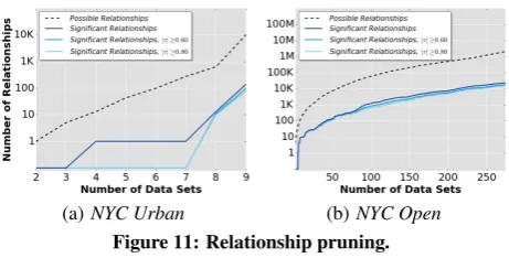
Figure 11: Relationship pruning.

tionship for 1,000 random spatial or temporal permutations. Also, the queries executed did not include any filtering clause. When us-ing a clauseC, the query evaluation step skips the significance test whenCis not satisfied, which further improves the performance.

Figure 10: Speedup Scalability.To test the scalability

of our framework, we computed the speedup attained by the diff er-ent componer-ents with increasing number of nodes in the cluster. This experiment was performed on Amazon Web Services (AWS) using theNYC Urbancollection. We used AWS because it allows the configurations of clusters of different sizes. Each node in the

cluster had an Intel Xeon E5-2670 v2 processor (8-core) and 61GB of RAM. Figure 10 shows the speedup for the three components of the framework, which was computed against the the time taken by a single node. A relatively lower speedup was attained for identi-fying features and evaluating relationships than for the scalar func-tion computafunc-tion. This is primarily due to the presence of straggler reducers that deal with higher spatio-temporal resolutions, thus in-creasing the computation time for the randomization tests.

Relationship Pruning. Figure 11 plots the the number of identi-fied relationships (in log scale), when considering the (week, city) resolution, with increasing number of data sets. For the data sets in

NYC Urban(Figure 11(a)), there was a significant decrease in the number of relationships—from 9,745 to 137, a decrease of about 98.60%. If we filter relationships havingτ≥0.6 andτ≥0.8, the reduction further increased to 99% and 99.20%, respectively. When handling a larger number of data sets, such as NYC Open, the advantages of our framework become even more evident, as Fig-ure 11(b) shows. Given the over 2 million possible relationships for the (week, city) resolution, our framework identified 22,327 of them to be statistically significant, which corresponds to a decrease of about 98.90%. Although the number of identified relationships is still large, this is significantly better than trying to make sense of over 2 million relations. In addition, we envision that users will ex-plore these relationships by searching, querying, and filtering them based on different attributes (e.g.,τ,ρ,α, space, and time).

6.2

Correctness and Robustness

Correctness.Most urban data sets have become available only re-cently and work on integrating them is still incipient [3]. Since

ex-treme weather conditions. Thus, if each year of data is modeled as a function (starting at the same day and time), a strong positive re-lationship should be observed for the two functions. This observa-tion was used to test our technique, which indeed identified the two functions to be strongly and significantly related across different resolutions. The relationship score and strength for the (hour, city) and the (hour, neighborhood) resolutions were (τ=0.99,ρ=0.85) and (τ=1,ρ=0.87), respectively.

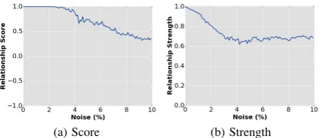
Robustness.To assess the robustness of our technique in the pres-ence of noise, we fixed a scalar functionf, and by artificially intro-ducing noise tof, we created a new (noisy) functionf∗. We used a random Gaussian noise where the amount of noise was bounded by a fraction of the inter-quartile range of the function. Note that noise was added to every spatio-temporal point of the function domain. We then evaluated the relationship between f and f∗. Figure 12 plots the relationship scores and strengths with increasing levels of noise added to the taxi density function. Note that even when the added noise was as large as 10% of the normal function range, we were still able to obtain a strong positive relationship (which was statistically significant) between the two functions. Further-more, the relationship score remained 1 even when the noise level was greater than 2%. This behavior can be attributed to the fact that topological persistence, which is used to identify thresholds for the salient features, is robust to noise [8]; small local maxima and minima, which are created due to the addition of noise, do not significantly affect the feature threshold.

6.3

Effectiveness: Interesting Relationships

We carried out a detailed study usingNYC Urbanto assess the ef-fectiveness of our approach at finding interesting relationships and pruning uninformative relationships that are not statistically signif-icant. In our evaluation, we found Weather to be the most polyg-amousdata set, being related through different attributes with all data sets in the collection, except Gas Prices, indicating the im-pact it has on different aspects of a city. We discuss some of these relationships below (additional relationships are described in Ap-pendix E.2). Unless otherwise noted, all relationships are with re-spect to salient features. Note that, while some of the results might imply the presence of a causal relationship, further analysis (not in the scope of this work) is required to ascertain causality.

Weather and Taxi. One of the relationships identified for the Taxi and Weather data sets in the (hour, city) resolution is be-tween the number of taxis and the average precipitation, having scoreτ=−0.62 and strengthρ=0.75. The values indicate a strong negative relationship: the higher the precipitation, the lower the number of taxis in the city. As discussed in Section 1, this con-firms the difficulty in finding taxis on a rainy day. When testing the hypothesis that this is due to taxi drivers being target earners, we found a positive relationship between average fare and precipi-tation (τ=0.73,ρ=0.7) implying increased earnings when it rains. Note that Farber [16] refuted this hypothesis since he did not find a correlation (using OLS regression) between the drivers’ earnings and rainfall. This is primarily due to two reasons: (i) he did not take into account the amount of rainfall—instead, he used a binary value indicating whether it rained or not; and (ii) more importantly, he considered the entire time period—periods with very sparse rain-fall are considered equivalent to those having higher rainrain-fall. Thus, this case study also provides evidence for the importance of look-ing at salient features, since they can evince relationships that are not visible when the whole data is taken into account.

While examining relationships involving extreme features, we found a negative relationship between the number of trips and the average wind speed. This relationship has a high score (τ=−1) and

(a) Score (b) Strength

Figure 12: Robustness evaluation using the density of taxi trips.

a low strength (ρ=0.13). The low strength is due to the presence of significant drops in the number of taxi trips at other periods, for example, during Thanksgiving, Christmas, and New Year [17] that are unrelated to the wind speed. However, the high score indicates that, whenever there is high wind speed, the number of taxi trips is significantly lower than usual, which is related to the impact of hurricanes in the city. We also found the same impact in the rela-tionship between number of unique taxis and average precipitation (havingτ=−1.0) when considering extreme features. It is worth noting that the number of taxi trips and wind speed are not related through salient features alone (also observed from Figure 1). This demonstrates the importance of computing relationships for salient as well as extreme features.

Weather and Citi Bike.We found a positive relationship between the average snow precipitation and the average bike trip duration in the (hour, city) resolution, havingτ=0.61 andρ=0.16. This im-plies that bike trips are longer in snowy days (or shorter when there is no snow), which is consistent with what we would expect. For a lower resolution—(day, city)—we found a negative relationship between the average snow precipitation and the active Citi Bike stations (τ=−0.88 andρ=0.65), i.e., fewer bike stations are used when it snows. We believe that this is related not only to the drop in bike usage under such weather, but also because heavier snow may impact certain stations more than others: the city clears snow at different frequencies depending on the location, and some stations may get cleared faster than others. Note that the latter relationship had a low score (τ=0) when considered at the higher resolution (hour, city): the impact is usually reflected only after the snow ac-cumulates, and such accumulation is not captured when using an hourly time step (higher resolution). This case illustrates the need for evaluating relationships at multiple resolutions.

Vehicle Collisions and Weather. We found interesting relation-ships between Vehicle Collisions and Weather, which correspond to the increased danger of accidents when it rains. There was a strong positive relationship between rainfall and number of mo-torists killed (τ=0.90,ρ=0.95) as well as number of injured pedes-trians (τ=0.75,ρ=0.66). However, we found no significant rela-tionship between number of accidents and rainfall, implying that, even though the number of accidents does not increase when there is heavy rain, their severity does. This leads to a new hypothesis that may explain the lack of taxis during rainfall: taxi drivers, be-ing experienced with the possible danger durbe-ing high rainfall, might return home during these periods.

Vehicle Collisions, 311, and Taxi.We identified relationships that involve the Vehicle Collision data set at the (hour, neighborhood) resolution: a strong positive relationship between the number of collisions and the number of 311 complaints (τ=0.99,ρ=0.86), and a strong positive relationship between the number of collisions and number of taxi trips (τ=0.99,ρ=0.79). While the implication of such relationships, especially the latter, is not clear, it provides a starting point for experts, pointing them towards data sets and attributes to be considered for further detailed analysis.

Effectiveness of Statistical Significance Test. Since there is no gold data available, to test the ability of the significance tests to re-move potentially uninformative relationships, we evaluated a ran-domly chosen set of statistically non-significant relationships. For instance, many relationships between the fare tax for taxi trips and different attributes from the Weather, 311, and 911 data sets were found not to be statistically significant. This indicates that, even though some of these relationship have|τ|>0.60, they are mostly random and coincidental. In fact, the tax charged in taxi trip fares does not have anything to do with different weather conditions, let alone with 311 and 911 complaints. Other examples of spurious re-lationships pruned by our framework include: mileage of taxi trips (Taxi) and number of injured pedestrians (Vehicle Collisions), hav-ingτ=0.90; number of bike trips (Citi Bike) and number of tweets (Twitter), havingτ=0.87; and number of 311 complaints and av-erage speed (Traffic Speed), havingτ=0.76.

We also computed the statistical significance for relevant rela-tionships using the standard Monte Carlo procedure. Many of these relationships were found to be not significant using this test, includ-ing the ones between the average snow precipitation and the aver-age bike trip duration. This underscores the importance of taking the spatial and temporal dependencies into account while assessing statistical significance.

Note that such tests represent a best-effort approach to identify candidate relationships, and thus, they can both return spurious re-lationships and miss important ones. Gold data are needed to quan-titatively study the trade-offs for the different techniques. Nonethe-less, our initial experiments indicate that these significance tests are useful and can help guide users in the data discovery process.

6.4

Comparison against Standard Techniques

We used theNYC Urban collection to compare our approach against established techniques for identifying dependencies between data: Pearson correlation coefficient (PCC) [7], mutual informa-tion (MI) criterion [33], and dynamic time warping (DTW) rou-tines [21, 31]. Some of these techniques are not naturally normal-ized for inter-dataset comparisons (e.g., DTW and MI) or directly extendable to spatio-temporal data. Thus, for this experiment, we proposed normalizations that provide a meaningful range of rela-tionship score (see Appendix D for details) and focused on data represented as a time series aggregated over the city resolution.

Overall, we observed that standard approaches can identify the basic relationships that are present across the entire data. For ex-ample, the relationship between average snow precipitation and Citi Bike trip duration could be detected by PCC as well as by MI. Sim-ilarly, the relationship between number of taxi trips and average traffic speed could be found using PCC and DTW. However, these techniques did not find relationships that are only visible under cer-tain conditions, such as the ones between rainfall and number of taxis, or wind speed and number of taxi trips. Also, relationships that take into account space, such as the ones between number of collisions and number of taxi trips, are not identified by any of the above techniques due to their inherent 1D nature.

7.

RELATED WORK

In addition to the approaches discussed in Section 6.4, other notions of relationship have also been explored by the data min-ing and data integration communities. Some methods focused on identifying relationships between data pointswithin a singledata set. Achtert et al. [1] focused on computing correlation clusters, which are composed of data points that present correlations be-tween different attributes. Yang et al. [37] used subspace cluster-ing, which finds different clusters of points for different subspaces of attributes, to identify relationships. Other methods have been proposed which identify different kinds of relationships. Sarma et al. [9] focused on finding candidate tables that can be unioned and joined, and considered such tables to be related. There has also been work ondata fusion, where relationships are sought between data sets that overlap or complement each other to resolve conflicts between different sources [10, 29] and to find their derivation his-tory [2]. These relationships are orthogonal to and can be used in conjunction with our technique to enrich the data discovery pro-cess. To the best of our knowledge, no existing method addresses the problem of identifying spatio-temporal relationships that take into account salient features in the data.

Recently, there has been a renewed interest in finding explana-tions for surprising results, oroutliers, in database queries [30, 36]. Scorpion [36] focused on understanding aggregate queries over a single data set. Roy and Suciu [30] handled more complex database schemas and proposed techniques that can be used to explain rela-tionships between different data sets. However, the thresholds for outliers must be specified by the user for each query, which be-comes impractical when handling hundreds to thousands attributes and without proper knowledge about the data sets. Since ourData Polygamyframework generates an overview of the relationships among different data sets, the approach proposed by Roy and Su-ciu [30] could be used to further explore and understand the most eye-catching relationships. Thus, the techniques complement each other in the data exploration process.

Methods for comparing scalar functions use topological abstrac-tions directly for this comparison (e.g., [4, 25]), due to which two functions are considered to be similar even if some affine transfor-mation of the functions are similar, i.e., spatio-temporal locations of the topological features are not considered. Unlike such meth-ods, we are interested in comparing scalar functions based on the spatio-temporal locations of their topological features.

8.

DISCUSSION AND FUTURE WORK

Scalar Functions.In this work, we mainly considered data whose spatial domain has dimension up to two. However, our framework is general and can handle higher dimensions as well. For instance, data corresponding to noise in buildings can be obtained in 3D, where in addition to geo-location, the noise level varies with height. By constructing an appropriate graph to represent this spatial do-main, the framework can be used as is.

While we have focused on numerical attributes, non-numerical attributes can be taken into account if they are mapped into numer-ical values (e.g., categornumer-ical values can be mapped to unique num-bers). In addition, while we chose to use the average to represent functions, it is straightforward to extend our framework to support other functions such assum,median,min, ormax. Alternatively, users can define custom functions as well.