warwick.ac.uk/lib-publications
A Thesis Submitted for the Degree of PhD at the University of Warwick
Permanent WRAP URL:
http://wrap.warwick.ac.uk/94785
Copyright and reuse:
This thesis is made available online and is protected by original copyright. Please scroll down to view the document itself.
Please refer to the repository record for this item for information to help you to cite it. Our policy information is available from the repository home page.
Nearshore Mixing due to the Effects of
Waves and Currents
By
Soroush Abolfathi
A thesis submitted in partial fulfilment of the requirements for the
degree of Doctor of Philosophy in Engineering
University of Warwick, Department of Engineering
i
C O N T E N T S
List of Figures vi
List of Tables xvi
Acknowledgements xix
Declaration xx
Contributions to Knowledge xxi
Notation xxii
Glossary xxvi
Abstract xxviii
1. INTRODUCTION 1
1.1Synopsis 1
1.2Aims and Objectives 2
1.3 Overview of the Thesis Structure 4
2. BACKGROUND THEORY AND PREVIOUS WORK 6
2.1 Synopsis 6
2.2 Nearshore Hydrodynamics 6
2.2.1 Wave Energy 7
2.2.2 Mass Transport and Momentum 8
2.2.3 Radiation Stress 8
2.2.4. Currents 9
2.3 Mixing and Dispersion Transport Processes in the Nearshore 12
2.4 Theory of Mixing 14
2.4.1 Molecular (Fickian) Diffusion 14
ii
2.4.3. Turbulence 19
2.4.4 Turbulent Diffusion 22
2.5. Transverse Mixing due to Wave Activity in the Nearshore Zone 24
2.5.1. Wave Theory 25
2.5.2. Wave-induced Currents 35
2.5.3. Turbulence in the Nearshore Region 42
2.5.4. Experimental Study of Transverse Mixing 55
2.6. Summary 68
3. THEORETICAL APPROACH 69
3.1 Synopsis 69
3.2 Mixing in the Nearshore 69
3.3 Theoretical Approach 77
3.4 Nearshore Mixing Processes 78
3.4.1 Turbulent Diffusion 79
3.4.2 Advective Shear Dispersion 83
3.5 Summary 92
4. MIXING UNDER COMBINED EFFECTS OF WAVES AND
CURRENT - LABORATORY MEASUREMENTS & ANALYSIS
93
4.1 Synopsis 93
4.2 Laboratory Investigations 93
4.2.1 Experimental Facility and Setup 95
4.2.2 Hydrodynamic Measurements 96
4.2.3 Wave Gauge Measurements 99
4.2.4 Fluorometric Measurements 100
iii
4.3 Experimental Data Analysis 104
4.3.1 Hydrodynamic Data 105
4.3.1.1 Primary Flow under Current Only Condition 105
4.3.1.2 Longitudinal Flow Velocity under Current Only Condition 106
4.3.1.3-Cross-Shore Velocity Profiles under Current Only Condition
107
4.3.1.4-Cross-Shore Velocity Profiles under Wave-Current Conditions
108
4.3.1.5 Wave Conditions 117
4.3.2 Solute Concentration Data 118
4.3.3 Mixing Coefficient of Fluorometric Study 128
4.4 Theoretical Model for Nearshore Mixing 132
4.4.1 Turbulent Kinetic Energy 133
4.4.1.1 Despiking Algorithm for LDA Data 136
4.4.1.2 TKE Algorithm 138
4.4.2 Turbulent Diffusion 147
4.4.2.1 Eddy Viscosity 147
4.4.3 Shear Dispersion 150
4.4.4 Comparison of Mixing with Existing Data 157
4.5 Summary 158
5. HYDRODYNAMICS MEASUREMENTS 161
5.1 Synopsis 161
5.2 Background 161
5.3 Experimental Setup 163
5.3.1 Calibration 166
iv
5.4 PIV Data Analysis 168
5.5 Hydrodynamic Results of the PIV Measurements 172
5.5.1 Velocity Field 172
5.5.2 Turbulence Decomposition 185
5.5.3 Turbulent Kinetic Energy 187
5.5.3.1 Comparison of Measured TKE with DHI Data 192
5.5.4 Turbulent Diffusion Mechanism 195
5.5.5 Shear Dispersion Mechanism 197
5.6 Summary 206
6. NUMERICAL SIMULATIONS 208
6.1 Synopsis 208
6.2 Motivation 208
6.2.1 Computational Fluid Dynamics 209
6.2.2 Grid-based Methods 210
6.2.3 Meshfree Methods 212
6.2.4 Meshfree Particle Methods (MPMs) 212
6.3 Smoothed Particle Hydrodynamics 213
6.3.1 SPH Method 215
6.3.1.1 Integral Interpolants 216
6.3.1.2 Smoothing Kernel (Weighting Function) 216
6.3.1.3 Governing Equations 219
6.3.2 Weakly Compressible SPH (WCSPH) Approach 219
6.4 The SPH Model Implementations 221
6.4.1 Density Re-Initialization Method 222
v 6.4.3 Time – Stepping Algorithm 224
6.4.4 Computational Efficiency 225
6.4.5 Initial Conditions 226
6.4.6 Boundary Conditions 226
6.4.7 Numerical Wave Generator 228
6.5 Numerical Results 229
6.5.1 Hydrodynamic Results of SPH Simulations 230
6.6 Application of the SPH Hydrodynamics in Nearshore Mixing 239
6.7 Summary 244
7. CONCLUSIONS 246
7.1 Future work 251
vi
L I S T O F F I G U R E S
Figure 2.1: Schematic of current pattern observed in the nearshore region under obliquely incident wave conditions……… 10
Figure 2.2: Schematic sketch of a nearshore circulation cell……….……… 11
Figure 2.3: Diffusive fluxes within small control volume of tracer, adapted from Rutherford (1994)………..………… 15
Figure 2.4: Reynolds’ stress eddy model, (Chadwick & Morfet, 1986)….... 21
Figure 2.5: Definition sketch of the generation of wind waves………..…… 26
Figure 2.6: Definition sketch for a small amplitude sinusoidal wave……… 27
Figure 2.7: Sketch depicting depth effects on particle orbits, (a) Deep water, (b) Water of intermediate depth, & (c) Shallow water, from Sorensen (1993)………. 31
Figure 2.8: Classification of wave breaking depth, (Horikawa, 1978)…….. 33
Figure 2.9: Classification of breaker types adopted from Horikawa (1978).. 34
Figure 2.10: Sketch depicting a typical Lagrangian velocity profile of the mass-transport in a progressive wave……….. 37
Figure 2.11: Vertical distribution of the non-dimensionalised Lagrangian velocity in a progressive wave (kd = 0.5, 1.0, 1.5), adopted from Longuet-Higgins (1953)………...……….. 38
Figure 2.12: Definition sketch of wave motion within the surfzone…….… 39
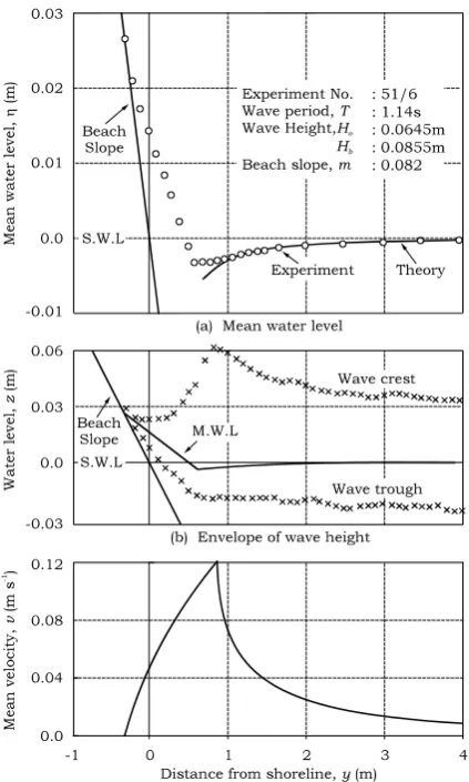
Figure 2.13: Example of (a) experimental results on wave up and set-down, (b) wave height envelope, and (c) Theoretical mean undertow
velocity……… 41
vii Figure 2.15: Comparison of longshore velocities measured by Galvin &
Eagleson (1965; Series II) with theoretical profiles derived by Longuet-Higgins (1970) , adopted from Longuet-Longuet-Higgins (1970) ………. 44
Figure 2.16: Measurement of turbulent kinetic energies under breaking waves in surfzone, adopted from Svendsen (1987) ……… 49
Figure 2.17: Measurement made by Nadaoka & Kondoh (1982) of turbulent intensities in the nearshore region ………. 52
Figure 2.18: Suggested sources of wave induced turbulence in the nearshore zone……… 54
Figure 2.19: On-off shore mixing characteristics for solute tracer studies in the surfzone (from Harris et al., 1963) ………..………. 57
Figure 2.20: On-off shore mixing characteristics for solute tracer studies in the surfzone (from Inman et al., 1971)……….…………..……..…….. 59
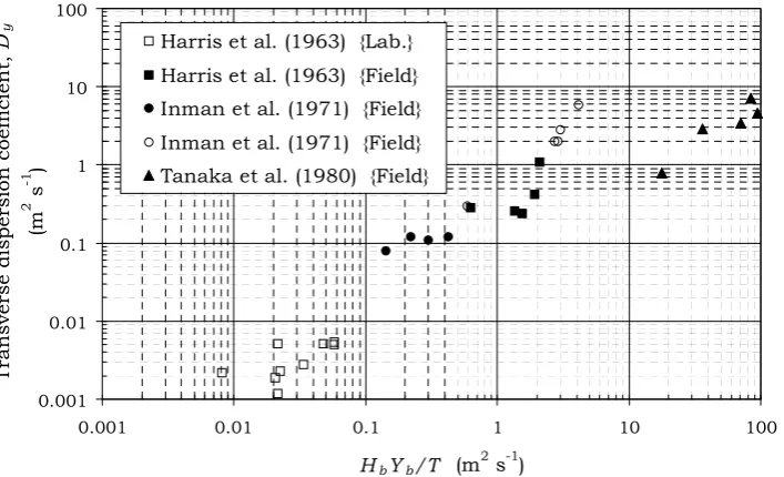
Figure 2.21: Transverse (on-off shore) mixing characteristics for tracer studies in the surfzone……… 60
Figure 2.22: Mixing characteristics for solute transport studies (from Bowden et al., 1974)... 64
Figure 2.23: Mixing characteristics for solute tracer studies adopted from Zeidler (1976)... 66
Figure 2.24: On-off shore mixing characteristics for solute tracer studies in the nearshore zone adopted from Elliott et al. (1997)…... 67
Figure 3.1: Schematic view of (a) wave-current interaction in the nearshore region (b) complex flow field due to the effects of wave and currents…….. 70
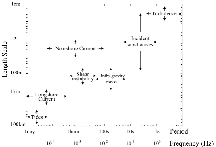
Figure 3.2: The temporal and spatial scales of hydrodynamic processes in the nearshore, adopted from Souza et al., (2014)……… 72
Figure 3.3: Schematic of circulation cells of longshore currents and rip
viii Figure 3.4: Definition sketch of mean horizontal velocity inside the
surfzone………..………. 84
Figure 3.5: Definition sketch of Zone dispersion model for (a) two zone model, (b) N zone model………. 88
Figure 4.1: Wave paddle system at large scale laboratory in DHI…………. 94
Figure 4.2: Layout of the Wave Current Basin at DHI, Denmark…………. 95
Figure 4.3: Wave guides/straighteners at downstream end of wave-current facility, DHI………..……….………. 96
Figure 4.4: Experiment coordinate system………. 97
Figure 4.5: (a) Laser Doppler Anemometry (LDA) system component, (b) LDA velocity measurement system, (c) laser probe installation inside the surfzone at DHI facility…..………. 98
Figure 4.6: Wave gauges configuration in DHI experiment………...……… 99
Figure 4.7: 10 AU Turnenr Design Fluorometer utilized in DHI experiment 100
Figure 4.8: Continous injection of Rhodamine WT dye in various locations across the nearshore... 101
Figure 4.9: (a) Sample extraction tubes in facility, (b) pumping system for
extraction………. 102
Figure 4.10: Typical calibration plot of fluorometer... 103
Figure 4.11: Longshore velocity profiles for current only condition at
x={3,6,9,15}m from flow inlet... 106
Figure 4.12: Longshore velocity profile for current only condition at y =
{2, 4 & 6}m from shoreline... 107
Figure 4.13: Cross-shore velocity in on-offshore direction at y = {2, 4 & 6}m for current only condition... 107
ix direction for Sop = 2% (a) inside the surfzone y={1,2,3}m (b) seaward of
the breaker region y={4,5,6}m... 109
Figure 4.15: Temporal averaged Cross-shore velocity in on-offshore direction for Sop = 3½ % (a) inside the surfzone y={1,2,3}m (b) seaward of
the breaker region y={4,5,6}m... 110
Figure 4.16: Temporal averaged Cross-shore velocity in on-offshore direction for Sop = 5% (a) inside the surfzone y={1,2,3}m (b) seaward of
the breaker region y={4,5,6}m... 111
Figure 4.17: Temporal averaged Cross-shore velocity in on-offshore direction for Sop = 3½ random% (a) inside the surfzone y={1,2,3}m (b)
seaward of the breaker region y={4,5,6}m... 112
Figure 4.18: Temporal averaged vertical velocity in on-offshore direction for Sop = 2% (a) inside the surfzone y={1,2,3}m (b) seaward of the breaker
region y={4,5,6}m... 113
Figure 4.19: Temporal averaged vertical velocity in on-offshore direction for Sop = 3½ % (a) inside the surfzone y={1,2,3}m (b) seaward of the
breaker region y={4,5,6}m... 114
Figure 4.20: Temporal averaged vertical velocity in on-offshore direction for Sop= 5% (a) inside the surfzone y={1,2,3}m (b) seaward of the breaker
region y={4,5,6}m... 115
Figure 4.21: Temporal averaged vertical velocity in on-offshore direction for Sop = 3½ Random% (a) inside the surfzone y={1,2,3}m (b) seaward of the breaker region y={4,5,6}m……….. 116
Figure 4.22: Wave height measurements across the nearshore region for all the wave conditions... 117
x Figure 4.24: Concentration for 3 injection points; surfzone, breaker point
and offshore Wave condition – monochromatic waves with H = 0.12m and
T=1.2sec……….. 121
Figure 4.25: Concentration for 3 injection points; surfzone, breaker point and offshore Wave condition – monochromatic waves with H = 0.12m & T
= 1.85sec………. 122
Figure 4.26: Concentration for 3 injection points; surfzone, breaker point and offshore Wave condition – monochromatic waves with H = 0.12m & T
= 2.9sec... 124
Figure 4.27: Concentration for 3 injection points; surfzone, breaker point and offshore Wave condition – monochromatic waves with Sop =
3½%Random ……….. 125
Figure 4.28: Relationship between the variance of the transverse concentration profiles and longitudinal distance for (a) current only condition, (b) Sop=2%, (c) Sop=3½%, (d) Sop=5% and (e) Sop=3½
Random%... 128
Figure 4.29: An example of velocity (u, w) records from LDA experiments – H = 0.12m & T = 1.2sec. (Top) measurements at 6m from SWL (Bottom) measurements inside the surfzone at 2m from SWL……….. 134
Figure 4.30: An example of on-offshore velocity (u) records for H = 0.12m & T = 1.2sec (Left) outside the surfzone, at 5m from SWL, (Right) inside the surfzoe, at 2m from SWL... 135
Figure 4.31: An example of multipoint spikes in LDA data - on-offshore velocity (u) records for H = 0.12m & T = 1.2sec outside the surfzone, at 4m from SWL……… 136
Figure 4.32: Pioncare map for the data with H = 0.12m & T = 1.2sec inside the surfzone, at 3m from SWL... 138
xi Figure 4.34: Variation of TKE over depth of water column across the
nearshore for the case of: (a) Sop=2%, (b) Sop=3 ½ %, (c) Sop=5% and (d)
Pseudo random waves... 142
Figure 4.35: Scarce on-offshore velocity records at 2m from shore and 5mm below the SWL for the case of H0= 0.12m and T = 1.85sec... 143
Figure 4.36: Comparison of TKE reported by Nadaokah & Kondoh (1982) with the DHI measurements for the case of a) Sop= 2%, b) Sop= 3½%, c)
Sop= 5% & d) Sop = 3½ Random%... 145
Figure 4.37: Comparison of measured eddy viscosity with Svednsen & Putrevu (1994) theoretical formulae... 149
Figure 4.38: Schematic of N-zone model for calculation of dispersive
mixing………. 151
Figure-4.39: Temporal Averaged undertow velocities for LDA measurements across the nearshore, a) Sop = 2%, b) Sop = 3½ %, c) Sop =
5%, d) Sop = 3½ Random%... 153
Figure 4.40: Comparison between shear dispersion coefficients obtained from undertow measurements with the dye measurements….……… 156
Figure 4.41: Comparison of on-off shore mixing in the surfzone…………... 158
Figure 5.1: Wave flume at Warwick Water Laboratory……….. 163
Figure 5.2: Schematic view of the PIV experimental setup……… 164
Figure 5.3: Schematic of experimental setup from the end of the tank view
point……….………… 165
Figure 5.4: Schematic representation of the imaging set-up in the PIV tests 166
Figure 5.5: (a) schematic sketch of calibration setup (b) calibration image... 166
xii Figure 5.7: Cross-correlation data processing procedure using an FFT
algorithm (a) defining the interrogation window to subsample the main sequential image pairs; (b) cross-correlation procedure with an FFT implementation; (c) identifying the peak’s location corresponding to the average shift of particles within the interrogation windows (d) converting the particle’s shift to physical space and calculating the velocity vectors…. 170
Figure 5.8: An example of PIV data processing (a) PIV unprocessed image (b) resultant velocity vector fields from processing... 171
Figure 5.9: Temporal variation of vector fields over a wave cycle at 3m from SWL for the case of monochromatic waves with Sop= 5%... 173
Figure 5.10: Temporal variation of vector fields over a wave cycle at 5m from SWL for the case of monochromatic waves with Sop= 5%... 175
Figure 5.11: Temporal variation of vector fields over a wave cycle at 3m from SWL for the case of monochromatic waves with Sop= 3½ %... 176
Figure 5.12: Temporal variation of vector fields over a wave cycle at 5m from SWL for the case of monochromatic waves with Sop = 3½%... 177
Figure 5.13: Temporal variation of vector fields over a wave cycle at 3m from SWL for monochromatic waves with Sop = 2 %... 179
Figure 5.14: Temporal variation of vector fields over a wave cycle at 5m from SWL for monochromatic waves with Sop = 2 %... 180
Figure 5.15: Temporal averaged horizontal and vertical velocity components of the PIV data for monochromatic waves with Ho = 0.12m
and T = 1.2sec………. 182
Figure 5.16: Temporal averaged horizontal and vertical velocity components of the PIV data for monochromatic waves with Ho = 0.12m
and T = 1.85sec……… 183
Figure 5.17: Temporal averaged horizontal and vertical velocity components of the PIV data for monochromatic waves with Ho = 0.12m
xiii Figure 5.18: Schematic of windowing technique for spatial averaging... 187
Figure 5.19: Definition sketch of Reynolds’ decomposition... 188
Figure 5.20: Temporal variation of TKE in offshore region {y=5m} for the monochromatic waves with Sop= 5%... 190
Figure 5.21: Temporal variation of TKE inside the surfzone {y=3m} for the monochromatic waves with Sop = 5%... 191
Figure 5.22: Comparison of the TKE obtained from the PIV and LDA measurements for the monochromatic waves with a) Sop = 5%, b) Sop = 3 ½
% and c) Sop = 2%……… 194
Figure 5.23: Comparison of the diffusivities ( ) obtained from the PIV and Theoretical approach proposed by Svendsen and Putrevu (1994)…………. 196
Figure 5.24: Schematic sketch of the dispersion mechanisms during a wave cycle based on the PIV data analysis ………. 197
Figure 5.25: Schematic of the shear dispersion mechanisms during a wave cycle and their temporal contribution based on the PIV data analysis……… 198
Figure 5.26: Temporal varioation of instantanious velocity profiles at 3m from SWL for the monochromatic waves of Ho = 0.12m and T = 1.2sec…. 199
Figure 5.27: Vertical distribution of spatially-averaged velocity over the full depth of FOV and centre of the PIV images for the monchromatic waves of Ho = 0.12m and T = 1.2sec in the breaker region (3m) and inner
surfzone (2m)………. 200
Figure 5.28: Temporal variation of shear dispersion across the nearshore for the monochromatic waves with Ho= 0.12m and T = 1.2sec……… 201
Figure 5.29: Temporal variation of shear dispersion across the nearshore for the monochromatic waves with Ho = 0.12m and T = 1.85sec…………. 202
xiv Figure 5.31: Comparison between the dispersion coefficient obtained from
the PIV data analysis and fluorometric study at DHI (§4.2.3)……… 205
Figure 6.1: Discretization approaches in CFD simulations, a) Eulerian b) Lagrangian methods……… 209
Figure 6.2: Sketch of the influence domain in SPH model……….. 217
Figure 6.3: Sketch of computational domain ……….……… 221
Figure 6.4: Neighbouring particles in two dimensional domain……….…… 226
Figure 6.5: Sketch of particle arrangement in wall boundary condition and the repulsive force between fluid and boundary particles………. 227
Figure 6.6: Two dimensional sketch of interaction between fluid and boundary particles……….. 228
Figure 6.7: Snapshots of SPH output for the case of monochromatic waves of Ho =0.12m and T = 1.2sec……….…… 231
Figure 6.8: Schematic illustration of temporal averaged velocity profiles from SPH output………. 232
Figure 6.9: Temporal-averaged on-offshore velocity profiles from SPH simulation for the waves of Sop = 5% at y = {1, 2, 3, 4 & 5}m……….. 233
Figure 6.10: Snapshots of SPH model output for simulation of monochromatic waves with H0 = 0.12m and T = 1.85sec……….. 234
Figure 6.11: Temporal-averaged on-offshore velocity profiles from SPH simulation for waves of Sop = 3½% at y = {1, 2, 3, 4 & 5}m……..………… 235
Figure 6.12: Snapshots of SPH model output for simulation of monochromatic waves with H0 = 0.12m and T = 2.9sec…..………. 236
xv Figure 6.14: Comparison between on-offshore temporal-averaged velocity
profiles of the SPH model and the LDA measurements for monochromatic waves of a) Sop=5%, b) Sop=3½% and c) Sop= 2%... 239
Figure 6.15: Schematic of velocity profile measurements from SPH simulations……….……. 240
Figure 6.16: Temporal variation of mixing coefficients obtained from SPH model for regular waves of Sop =5% at a) surfzone [2m], b) breaker region [3m], c) offshore [5m]………. 242
Figure 6.17: Comparison between the overall mixing coefficients determined for the SPH model and the tracer measurement data…………... 244
Figure 7.1: Schematics of wave mechanisms within a wave cycle…….…… 247
Figure 7.2: The diffusive and dispersive mixing mechanisms for the monochromatic waves with Sop = 5%... 249
Figure 7.3: The diffusive and dispersive mixing mechanisms for the monochromatic waves with Sop = 3½%... 249
xvi
L I S T O F T A B L E S
Table 2.1: Asymptotes of wave functions……… 29
Table 2.2: Classification of breaker types (from Galvin, 1972) ……… 34
Table 4.1: Summary of experimental studies at DHI……….. 103
Table 4.2: Measured wave conditions in the offshore region of basin
(y=6.5m)……….. 117
Table 4.3: Transverse mixing results for a continuous injection of tracer inside the surfzone, 2m from the shoreline under waves of varying T, with an Ho =0.12m………... 131
Table 4.4: Transverse mixing results for a continuous injection of tracer at breaker region, 3m from the shoreline from the shoreline under waves of varying T, with an Ho =0.12m ……… 131
Table 4.5: Transverse mixing results for a continuous injection of tracer, 5m from the shoreline from the shoreline under waves of varying T, with an
Ho =0.12m……… 132
Table 4.6: Comparison of the shear dispersion coefficients determined with
N-zone model (undertow values and depth-averaged t) with the dye
measurements……….. 154
Table 4.7: Comparison of the shear dispersion coefficient determined with
N-zone model (undertow values and depth-varying t) with the dye
measurements……….. 154
Table 5.1: Summary of the PIV test conditions, Warwick Water Lab (2014) 167
Table 5.2: Comparison between obtained from temporal variation of
xvii Table 5.3: Comparison between obtained from temporal variation of
shear dispersion and DHI tracer measurements for monochromatic waves with Sop = 3½ % ………..… 204
Table 5.4: Comparison between obtained from temporal variation of
shear dispersion and DHI tracer measurements for monochromatic waves with Sop = 2%...……….. 204
Table 6.1: Governing equations of fluid motion in Eularian and Lagrangian description (adopted from Liu & Liu, 2003) ………..…… 210
Table 6.2: Comparison of Lagrangian & Eulerian methods, (adopted from Liu & Liu, 2003) ………. 211
Table 6.3: Meshfree methods in chronological order (Liu & Liu, 2003)….. 212
Table 6.4: Meshfree particle methods (adopted from Liu & Liu, 2003)…… 213
Table 6.5: Recent applications of SPH in coastal engineering related
problems……….. 215
Table 6.6: Summary of kernel options in the SPH and their formulations…. 218
Table 6.7: SPH formulation for conservation laws of fluid motion……… 219
Table 6.8: Simulation test cases for the SPH model………... 221
Table 6.9: Summary of the numerical technique implemented for the SPH
simulations……….….. 229
Table 6.10: The dispersion coefficients of the SPH simulations for the monochromatic waves with Ho = 0.12m and T = 1.2sec………. 243
Table 6.11: The dispersion coefficients of the SPH simulations for the monochromatic waves with Ho = 0.12m and T = 1.85sec……….. 243
xviii
D E D I C A T I O N
I would like to dedicate this thesis to my beloved parents, Ali and Nasrin for their
unconditional love and for their selfless and invaluable support throughout my
xix
A C K N O W L E D G E M E N T S
The completion of this doctoral thesis would not have been possible without the guidance and support of the kind people around me. Above all, I would like to thank my family for their unconditional support over the past years.
This work would not have been possible without the help, invaluable criticism and advice of my principal supervisor, Dr. Jonathan Pearson, not to mention his valuable knowledge and expertise in the field of coastal engineering. I would like to thank Dr. Pearson for his willingness to spend much time supervising this project. Thank you for keeping me going when times were tough. Also, I must express my gratitude to my co- supervisor, Professor Ian Guymer for his invaluable support, scientific advice and encouragement throughout my time at Warwick.
I am indeed grateful to School of Engineering, University of Warwick for offering me a Ph.D. Scholarship which provided me with the financial support.
xx
D E C L A R A T I O N
I hereby declare that this thesis is all my own work except where I have otherwise
stated and that this thesis has not been submitted for a degree at any other University.
Soroush Abolfathi
xxi
C O N T R I B U T I O N S T O K N O W L E D G E
Peer Reviewed conference proceedings.
1. ABOLFATHI S., PEARSON J. M., 2014. Solute dispersion in the nearshore
due to oblique waves. Proc. of Coastal Eng. 1(34).
2. ABOLFATHI S., PEARSON J. M., 2016. A Lagrangian Particle-based
models in Nearshore Mixing: A comparison to Laboratory Data, Proc. of
Coastal Eng. (Accepted, In press)
Conferences
1. ABOLFATHI S., PEARSON J. M. & GUYMER I., 2014. Modelling mixing mechanisms in the nearshore. International Association of Hydro-Environment Engineering & Research, Coventry, UK. [Oral & Poster presentation]
2. ABOLFATHI S., PEARSON J. M. & GUYMER I., 2014. Pollution at the seaside: Mixing due to the effects of waves and currents. YCSEC (10), Cardiff, UK. [Best presentation prize, considered for publications in Journal of Maritime Eng., ICE]
3. ABOLFATHI S., PEARSON J. M., 2014. Solute dispersion in the nearshore due to oblique waves. International Conference on Coastal Engineering, ASCE, Seoul, South Korea. [Oral presentation]
Prizes and awards
- Young Coastal Scientist Award, YCSEC (2014)
- Travel Grant, School of Engineering, the University of Warwick (2014) - Research Consumable grant, School of Engineering, the University of
Warwick (2013)
xxii
N O T A T I O N
Lower case
a wave amplitude [m]
b local dispersion coefficient [m2/s]
c concentration of diffusant [ml/l]
d total water depth [m]
dtr depth to wave trough level [m] em molecular diffusion coefficient [m2/s] e diffusion coefficient [m2/s]
ewf turbulent diffusion generated by oscillatory wave motion [m2/s] g gravitational constant = 9.81m/s2[m/s2]
g Group velocity [m/s]
k wave number 2π/L [m-1]
kx longitudinal dispersion coefficients [m2/s] ky transverse dispersion coefficients [m2/s] l length [m]
m beach slope
n dimensionless ratio of wave group velocity to wave phase velocity
q fractional thickness
qw maximum orbital velocity [m/s]
R2 least-squared linear regression coefficient
so bed slope
t duration or time [s]
u velocity in x-direction (varying with time) [m/s]
us surface velocity in x-direction [m/s]
u* local bed shear velocity in x-direction [m/s] v velocity in y-direction (varying with time) [m/s]
v* local bed shear velocity in y-direction [m/s]
v+ temporally averaged velocity in crest-trough level [m/s] v- temporally averaged undertow velocity[m/s]
va mean amplitude velocity [m/s]
w velocity in z-direction (varying with time) [m/s]
x horizontal distance, in direction of wave propagation [m]
xxiii
z vertical distance, origin at water surface [m]
zo bottom roughness parameter [m] zδ displacement parameter [m] Upper case
A total cross-sectional area [m2]
B diffusion velocity [m/s]
Bb breaker coefficient
C velocity of wave propagation (celerity) [m/s]
C Chezy bed frictional coefficient [m1/2/ s]
D shear dispersion coefficient [m2/s]
Db wave energy dissipation per unit area E overall mixing coefficient [m2/s]
E total wave energy [J]
F fluorescent intensity
H wave height – distance from crest to trough [m]
Hs significant wave height [m]
J diffusive flux [m/s]
I temporal wave-averaged momentum [kg/m s]
K reflection coefficient
Ke turbulent kinetic energy [m2/s] L wave length [m]
Lm length scale [m] N arbitrary constant
P non-dimensional parameter
P wave power per unit crest length [kW/m]
Q mass of tracer [kg]
Qb fraction of the breaking waves Rw dimensionless wave parameter
Re Reynolds number
S radiation stress [N/m2]
T wave period [s]
Ts significant wave period [s]
V temporally averaged (over wave cycle) drift velocity [m/s]
xxiv Greek Letters
γ breaker depth index δ wave steepness = H /L
η vertical displacement of water surface from mean surface elevation at z
= 0 [m]
κ von Karman universal constant λa relative acceleration threshold
μ dynamic viscosity [kg/m s] μ position of centroid [m] ν kinematic viscosity [m2/s] νt eddy viscosity [m2/s]
coefficient of proportionality
θ angle [degree]
ϕ Vertical distribution function π 3.1416
ρ fluid density [kg/m3]
σ standard deviation
σ2 spatial variance [m2] τ viscous shear stress [N/m2] τo bed shear stress [N/m2]
ω wave angular frequency =2π/T [s-1] Subscripts
+ onshore direction - offshore direction
b breaking conditions
c current
d spatially depth averaged
i oscillatory flow
o deep water conditions
os oscillatory flow
t turbulent property
tc tidal current
T total
w wave
xxv
y transverse direction
z vertical direction Other notation
u´ e.g. u prime, denotes turbulent fluctuation of velocity
͞
xxvi
G L O S S A R Y
ADV Acoustic Doppler Velocimetry
BC Boundary Condition
CFD Computational Fluid Dynamics
EFG Element Free Galerkin
FD Finite Difference
DEM Discrete Element Method
FEM Finite Element Method
FLIC FLuid-In-Cell
FOV Field Of View
FPS Frame Per Second
FVM Finite Volume Method
LBE Lattice Boltzmann Equation
LDA Laser Doppler Anemometry
LDV Laser Doppler Velocimetry
MAC Marker-And-Cell
MLPG Meshless Local Petrov-Galerkin
MLS Moving Least Square
MPM Meshfree Particle Methods
MWS Mesh-free Weak-Strong form
xxvii PIC Particle-In-Cell
PIM Point Interpolation Method
PIV Particle Image Velocimetry
PPM Part Per Million
PPB Part Per Billion
RMS Root Mean Square
SF Scale Factor
SPH Smoothed Particle Hydrodynamics
SWL Still Water Line
TKE Turbulent Kinetic Energy
xxviii
A B S T R A C T
Analytical, experimental and computational studies were carried out to investigate the mixing and dispersion of neutrally buoyant tracer in the nearshore region due to the effects of waves and currents. The main objective of this study was to quantify the mixing processes in the nearshore region.
Theoretical approaches were developed to quantify the contribution of diffusive and dispersive mixing in the nearshore due to wave activity. An analytical model was developed to quantify the diffusive and dispersive mixing mechanisms based on mathematical solutions for the advection-diffusion equation.
Mixing under the combined effects of waves and currents were studied through measurement of hydrodynamic and fluorometric tracing experiments from a large-scale facility at the Danish Hydraulic Institute, Denmark. The experiments were conducted in a shallow water basin for a range of hydrodynamic conditions covering wave steepness between 2 – 5%. Data from detailed measurements were used to examine the spreading of a solute inside the surf zone and seawards of the breaker region. The overall depth-averaged on-offshore mixing coefficient obtained from the hydrodynamic experimental studies were compared to the mixing coefficients determined from the tracer measurements. It was shown that inside the surfzone, the shear dispersion is the dominant mixing factor, which is almost an order of magnitude greater than the diffusive mixing. The location of the breaker point and the wave height across the nearshore is shown to be important for determining the mixing coefficient.
Further detailed spatial and temporal variations of flow hydrodynamics across the nearshore were investigated through a series of laboratory experiments with the use of Particle Image Velocimetry. The experiments were undertaken in a dedicate wave flume at the University of Warwick. Through analysis of the PIV data, new information on the spatial variation of diffusion and dispersion in the shallow water column of the nearshore region was obtained. Flow visualisation of the PIV results identified three distinct hydrodynamic processes during the bore, undertow and the bore/undertow interaction, which were the primary mixing mechanisms in the nearshore region. The temporal variation of dispersion coefficient shows that intense shearing mechanisms exist during wave bore/undertow interactions.
The numerical capabilities of Smoothed Particle Hydrodynamics, a Lagrangian, meshless, particle-based method in modelling the nearshore hydrodynamics were explored in this study. The numerical data was used to quantify the mixing processes.
xxx
"When I meet God, I am going to ask him two questions: Why relativity? and why turbulence? I really believe he will have an answer for the first."
1
CHAPTER 1
INTRODUCTION
1.1
Synopsis
The nearshore zone experiences pollutant loading through both the shoreline and seaward boundaries. From the seaward boundary, pollutant loading is transported landward towards the surfzone by the so-called Stokes drift effect (Stokes, 1847). From the shoreline boundary, runoff pollution, which can contain faecal indicator bacteria and human viruses (Schiff et al., 2003) can drain into the surfzone. Consequently, pollution can congregate in the nearshore region, and as such, the water quality can affect the health of the general public who frequent beaches and thus is seen as a global problem (e.g. over a million beachgoers visit Santa Monica Bay beaches on a typical summer weekend – Schiff et al., 2003). However, the key mass exchange processes related to the pollutant transport and dilution within the nearshore water body are still not fully understood.
2 The nearshore zone is subject to a combination of both wave and longshore currents. This results in a complex three-dimensional flow field which is affected by the surface and bed generated turbulence, orbital motions of the wave, spatial variation of flow depth and vertical and transverse shear effects caused by longshore currents activities.
Although several field and laboratory studies have been undertaken to understand the mixing processes within the nearshore zone, quantifying all associated parameters are challenging due to the measurement limitations in this region. This project is specifically focussed to improve understanding and technical descriptions of the dispersal of neutrally buoyant pollutants. Through a range of theoretical, experimental and numerical investigations, the mixing processes under a range of wave-only and wave-current conditions are quantified.
1.2
Aims and Objectives
3 The objectives of this study are to elucidate the underlying mechanisms that leads to the mixing of neutrally buoyant pollutants in the coastal waters under different hydrodynamic conditions and to quantify those mixing mechanisms inside the surfzone as well as seaward of the breaker region, by use of experimental and numerical studies. In addition, this project aims to identify the current lack of knowledge in the theoretical modelling of wave mixing in the coastal region by identifying and studying those effective mechanisms in the nearshore, in order to provide a better understanding of the underlying physics of solute mixing and transport in coastal waters. The specific objectives of this research work are as follows:
1. To develop a theoretical approach for quantifying wave mixing parameters in the nearshore region.
2. To study mixing of buoyant pollutant under wave-current conditions for the first time, by critically analysing hydrodynamic and fluorometric data from large scale laboratory measurements, undertaken in shallow water basin of Danish Hydraulics Institute, Denmark in 2005 (Pearson et al., 2006). The data collection study measured a range of wave steepness and the dataset was used to examine the associations between the proposed theoretical mixing mechanisms with measured hydrodynamics and fluorometric data, identified in this study. Specifically to determine:
a. The overall mixing coefficient from analysis of the fluorometric data.
b. The Turbulent Kinetic Energy (TKE) and turbulent diffusion coefficient (ey) for the hydrodynamic data.
c. The overall shear dispersion coefficients (Dy) for the hydrodynamic
data.
4 a. The temporal and spatial variation of diffusion coefficients across the
nearshore
b. The temporal and spatial variation of dispersion coefficient across the nearshore
4. To validate the proposed theoretical model and mixing parameters with the state-of-the-art Lagrangian meshless particle-based numerical approach, developed within this study.
1.3
Overview of the Thesis Structure
This thesis comprises seven chapters:
In Chapter 2 (Background theory and previous work), an overview of nearshore hydrodynamics and mixing under the effects of waves and currents is presented. A detailed review of the published literature on the fundamental theories and the previous work on different aspects of mixing in the nearshore is presented.
In Chapter 3 (Theoretical approach), a theoretical approach is developed to quantify the nearshore mixing under different hydrodynamic conditions.
5
Chapter 5 (Hydrodynamic measurements) presents the results of the laboratory measurements performed in the Warwick University wave flume. The experiments were carried out to measure the hydrodynamic field in the nearshore region using Particle Image Velocimetry. The experiments presented in this chapter cover hydrodynamic conditions similar to the DHI experiment (Chapter 4). The hydrodynamic flow field obtained from the PIV measurements is utilized to demonstrate a revised mixing mechanisms which are present within a wave cycle. This provides an improved understanding of mixing processes in the nearshore due to the turbulence and shear dispersion.
In Chapter 6 (Numerical approach), Lagrangian particle-based, Smoothed Particle Hydrodynamics (SPH) capabilities are employed to model the hydrodynamic behaviour of the flow in the nearshore region. This section covers the methodology of SPH numerical methods, the modelling procedures and application of SPH in quantifying the mixing mechanisms.
6
CHAPTER 2
BACKGROUND THEORY AND PREVIOUS WORK
2.1 Synopsis
This chapter discusses nearshore hydrodynamics and its influence on the mixing in the nearshore due to the effects of waves and currents. The governing equations and underlying concepts are reviewed and discussed to understand the mixing and dispersion mechanisms in the nearshore environment. A detailed review of the previous theoretical, experimental and numerical studies conducted on mixing, dispersion and diffusion is discussed.
2.2 Nearshore Hydrodynamics
Nearshore hydrodynamics is a highly intricate topic in the field of coastal engineering that addresses waves and wave generated phenomena within the nearshore region. Waves breaking on a sloping beach near to the shoreline can release large amounts of energy which is predominantly expressed as turbulence in the water column (Svendsen & Putrevu, 1994). As waves approach the shore, the wave height and the wave momentum will reduce, while the wave interactions with the bottom topography significantly increase due to frictional effects. This transfer of momentum instigates the formation of longer period waves and currents (Svendsen & Putrev, 1996) that ultimately drive processes such as mixing and dispersion within the surf zone.
7
2.2.1 Wave Energy
Coastal processes are mainly influenced and derived by the energy of the incident waves in the surfzone. Airy theory (1845) describes the energy of a wave, based on the displacement of water particles due to the wave motion. Airy (1845) theory states that as a wave passes through a point the particles in that location will be displaced, moving through an orbit that is dependent on water depth, before returning to their original position and hence not resulting in a net displacement of mass. The shape of the orbital path traversed by a particle varies with water depth, it has circular path offshore, while elliptical in shallow water. The wave energy could be defined as the sum of its potential and kinetic energies. The potential energy of a wave is a function of the variation in the free surface elevation of the water body due to the motion of the wave whilst the kinetic energy is derived from the orbital motion of the particles under the wave (Komar, 1998). In order to derive total energy density of waves, these factors should integrate over the wave length (Eq. 2.1).
L L h u w dzdx
L dzdx gz L E
0 0
2 2
0 0
) (
2 1 1 )
(
1
(2.1)
where L is wave length, η is water surface elevation. Wave energy density E, will not remain constant while it travels towards the shallow water region and consequently breaks. Equation 2.1 indicates that energy density is very dependent on the wave height, which varies significantly during transition from offshore region towards the surfzone. The energy flux P, is the total energy of the wave which follows the laws of conservation of energy and opposed to the energy density E within the wave (Eq. 2.2).
g
EC ECn
P (2.2)
where C represent the celerity, Cg is the group velocity and n is a dimensionless ratio
8
2.2.2 Mass Transport and Momentum
One of the key flaws in the linear Airy theory is the assumption of particle motion in a closed circular or elliptical orbit. This assumption does not take into account the mean motion of the water in the surfzone towards the shoreline (Dean & Dalrymple, 2002). The elliptical particle orbits, actually involve a net shoreward progression in the nearshore region and therefore the particle motion path is not a closed loop. Mass transport towards the shoreline can be estimated according to equation 2.3.
2
1 1 2
) , (
1 t
t h u x z dzdt
t t
M (2.3)
Dean & Dalrymple (2002) pointed out that evaluation of M for the mean water surface level will be zero. Equation 2.3 clearly shows that the mass transport in the direction of wave propagation is non-linear. Also, it shows that the mass transport of the waves with a higher energy content will be higher. Mass transport always has momentum associated with it, which could be defined according to equation 2.4.
2
1 1 2
) ) ((
1 t
t h u u dzdt
t t
M (2.4)
The transfer of momentum through the wave breaking process results in a force known as radiation stress (§2.2.3).
2.2.3 Radiation Stress
9 )
( 2 1 2
1 2
gh S g h
M xx
] ) sin( [
kh kh E
Sxx (2.5)
The radiation stress is denoted by Sxx, the x axis is placed in the direction of wave
advance whilst the y axis is parallel to the breaker line, is the mean water level
set-down in the trough offshore from the breaker line.
2.2.4. Currents
Nearshore currents are primarily driven by waves that are incident on the coastal region; however, tidal fluctuations and winds blowing in the longshore direction can also influence current magnitudes (Komar, 1998). The study of currents in the coastal region is a key concept in the determination of transport, mixing and dispersion of pollutants in the nearshore, as they could have direct impact on these processes. The total current in the nearshore zone can be represented as the sum of a number of forcing mechanisms, each acting on different scales, as shown in equation 2.6.
i os b tc
w u u u u
u
u (2.6)
The above equation represents the steady current u as the sum of the breaking waves action ub, currents driven by strong local winds uw, tidal current utc, infra-gravity
waves ui and oscillatory flows due to wind driven waves uos (US Army Corps, 2002).
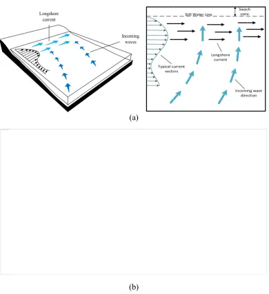
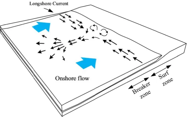
10 There are two primary quasi-steady current systems, the first of which is the longshore currents and the second one is the rip currents. Longshore currents propagate parallel to the shore in the nearshore zone and are driven by waves approaching the shoreline at an oblique angle. The nearshore current system developed by obliquely incident waves is shown in Figure 2.1.
Figure 2.1 – Schematic of current pattern observed in the nearshore region under obliquely incident wave conditions
The longshore current (Fig. 2.1) is generated by changes in the momentum flux of the wave field in the alongshore direction, resulting in a transfer of momentum from the wave field to the mean longshore current (Johnson, 2004).
Rip currents are also classed as quasi-steady currents. Rip currents are strong, narrow offshore directed flows that pass through the surf zone often carrying sediment and debris that discolours the water compared to adjacent areas (Komar, 1998; Brander 1998, Short 1985). Rip currents are formed primarily due to longshore variations in radiation stress, the resulting imbalance of which between the free surface set-up and the radiation stress induces a region of narrow offshore directed flow. Figure 2.2 shows schematic of features driving rip current flow in the nearshore region, resulting in a nearshore circulation cell. Nearshore circulation cells are constrained within the surf zone, however their lengths are variable, with the spacing between rip
Ty
pic
al
c
ur
re
nt
d
ist
ri
bu
tion
(p
la
ne
b
ea
ch
)
Oblique angle of wave approach driving longshore currents
11 features ranging from one to eight times the width of the surf zone (Inman et al., 1971). Nearshore circulation cells are responsible for a continuous flow of water between the surf zone and the offshore zone and act as distributing mechanisms for contaminants present within the surf zone (Inman et al., 1971).
Figure 2.2 – Schematic sketch of a nearshore circulation cell
Variable currents are one of the nearshore circulation mechanisms which display flow with frequencies lower than the incident wave climate, but with a higher level of variability than the quasi-steady currents active in areas which are restricted by the incident wave climate and or topography (Svendsen, 2005). There are two classes of variable nearshore waves; infragravity waves and shear waves.
Infragravity waves are oscillations in the water level within the surf and swash zones that occur due to long period variations in the wave set-up caused by the passage of wave groups. A variety of energetic infragravity waves exist within the nearshore zone with periods of between 20 and 200 seconds including edge waves and surf beat (Johnson, 2004; Olsson, 2004; Svendsen & Putrev, 1996). Long period infragravity waves generally form standing waves on sloped beaches due to their low wave steepness (Horikawa, 1988).
Shear waves are another infragravity effect that can influence the magnitude of longshore currents. Shear waves are low frequency, wave like oscillations of longshore currents with periods and wavelengths of 100 seconds and 100 metres
Longshore currents
Beach
Ri
p C
ur
ren
t Breaker Zone
Ri
p C
ur
ren
t
12 respectively (Svendsen & Putrev, 1996). They are driven by the incidence of large waves upon the shoreline causing an oscillation in the velocity of flow within the longshore at a low frequency (Dean & Dalrymple, 2002). Shear wave motion relies on the action of cross-shore shear as a restoring force rather than gravity (Bowen & Holman, 1989; Dean & Dalrymple, 2002). This motion occurs in the horizontal plane and causes the longshore current to move back and forth across the surf zone. The total velocity variance in the longshore current due to the action of the shear waves can exceed that due to other infragravity effects such as edge waves or surf beat (Howd et al., 1991; cited in Johnson, 2002). It has also been suggested by Kirby
et al. (1998) that resonant interactions may exist between shear waves and the other infragravity effects.
2.3 Mixing and Dispersion Transport Processes in the
Nearshore
Mixing and dispersion are key transport processes within coastal waters and the surf zone. They are critical parameters to consider when investigating the ability of coastal waters to receive and dilute discharged material (List et al., 1990).
13 responsible for a continuous interchange of water between the nearshore and offshore regions. As such they are key dispersal mechanisms for material injected into the surf zone. The intensity, frequency and direction of the incident wave climate, as well as the dimensions of the nearshore circulatory cells, have been found to be key variables impacting on the nearshore mixing processes (Inman et al., 1971).
The terminology used to describe mixing and dispersion in this research are defined according to Fischer et al. (1979). Some of the key mechanisms and their definitions are listed below:
● Mixing: Any process that leads to one parcel of water becoming intermingled with, or diluted by another, referring specifically to the action of dispersion and diffusion.
● Dispersion: The process of scattering particles or a cloud of contaminants through the combined effects of shear and transverse diffusion.
● Diffusion (Turbulent): The random spreading of particles through turbulent motion. Turbulent diffusion is considered to be somewhat analogous to molecular diffusion; however the scales of motion, described by ‘eddy’ diffusion coefficients, are significantly larger.
● Diffusion (Molecular): Refers to the scattering of particles through random molecular motion. This is described by Fick’s Law of diffusion (Eq. 2.7), where q
represents the solute mass flux, c is the mass concentration of a diffusing solute and is the co-efficient of proportionality also known as the molecular
diffusivity.
x c q
(2.7)
● Advection: transport due to an imposed current system, including quasi-steady and variable currents in the nearshore region.
14
2.4 Theory of Mixing
In this section, the role of molecular diffusion within aqueous related studies is considered, initially in a stationary fluid, and then examined whilst moving. The diffusion is modelled using a concentration gradient process based on an analogy to Fick’s (1855) first Law. As pointed out by Fischer et al. (1979), molecular diffusion when considered by itself in hydraulic related studies is insignificant, and in many laboratory and field studies is assumed to be negligible. However, the mixing enhanced by other additional processes is considered to strongly resemble molecular diffusion albeit on a larger scale.
2.4.1 Molecular (Fickian) Diffusion
Consider a small parcel of neutrally buoyant tracer placed in still water, a large distance from any boundaries. With time the tracer spreads slowly and equally in all directions. The spreading of the tracer is known as molecular diffusion and results from the random molecular motion occurring within the fluid, the so-called Brownian motion effect, first observed by the botanist Robert Brown and developed statistically by Einstein (1905).
In 1855, Fick reported an analogy which related the molecular diffusion of salt in water to the diffusion of heat along a metal rod, described by Fourier’s law of heat flow. Fick’s law states:
The rate of mass transfer of a diffusion substance through a unit area of an isotropic media is proportional to the concentration gradient measured normal to the section.
When considered in one dimension, Fick’s Law can be described mathematically by
x c e
Jx m
15 where Jx denotes the rate of molecular transport across the unit area (molecular
diffusive flux); c the concentration of the diffusion substance; x the distance normal to the area across which the material is transported; and em the molecular diffusion
coefficient. The minus sign indicates that diffusion occurs from a region of higher concentration to lower concentration.
Rutherford (1994) pointed out that although Fick’s law is based on a hypothesis rather than an actual physical description, empirical studies show that the relationship between the molecular diffusive flux, Jx and the concentration
gradient,c x, defined in equation 2.8 are remarkably linear. The molecular
diffusion within a fluid is dependent on density and temperature. Typical values of molecular diffusion, determined empirically in water, lie in the range
1 2 9m s
10 0 . 2 5 .
0 (Rutherford, 1994).
Consider a very small parcel of tracer within a fluid, as illustrated in figure 2.3. The control volume has the dimensions x,y&z ; the passage of molecules, or
diffusive fluxes, entering the control volume through the boundaries located at x, y, z
is given by Jx,Jy&Jz; and the diffusive fluxes leaving the parcel of fluid located at
z z y y x
x , & are given by Jxx,Jyy &Jzz. By definition, the mass of
tracer, Q within the control volume at time t, may be given by
z y x c
Qt t (2.9)
where ct = the average concentration within the parcel of fluid at time t.
16 After a small time interval, t at time, tt , let the mass be denoted by Qtt. By
the application of the law of conservation of mass, during the time interval, t the
rate of change of mass in the control volume may be given by (Rutherford, 1994):
t Q Q
t
Q t t t
(2.10)
By recalling the law of conservation of mass, the passage of molecules into and out of the control volume during the time interval, t must equalQ t, thus
(Rutherford, 1994): y x J J z x J J z y J J t Q z z z y y y x x
x
) ( ) ( ) ( (2.11)
For simplicity, consider the passage of molecules into the control volume in the x -direction only. From equation 2.8, the diffusive flux into the control volume, through the surface A, yields Jx em
c x
. Now consider the diffusive flux leaving thecontrol volume through surface B. The diffusive flux, Jxx can be evaluated by
adopting a Taylor’s series expansion. By assuming that the time interval, t is small,
the second and higher order terms can be neglected. This leads to the result (Rutherford, 1994):
x x J J
Jx x x x
(2.12)
17 z y x x c e x z y J
Jx x x m
) ( (2.13)
Equation 2.9 defines the mass of the tracer within the control volume, it is noted that the volume is constant, thus by adopting equation 2.9 and recalling the law of conservation of mass, leads to the result
z y x t c t
Q
(2.14)
So far, consideration of the passage of molecules entering and leaving the control volume has been restricted to the x direction only, however the same analytical procedure can be applied to the other two orthogonal directions. Combining equations 2.12, 2.13 and 2.14, and by recalling that in homogenous, isotropic conditions, the tracer spreads equally in all directions, enables the ‘classical diffusion equation’ to be derived (Rutherford, 1994):
2 2 2 2 2 2 z c y c x c e t c m (2.15)
2.4.2 Advective Diffusion
So far, it has been assumed that the parcel of fluid has been stationary and spreading of the tracer is generated by molecular diffusion alone. In an extension to the previous result (Eq. 2.15), now consider the movement of the control volume in laminar flow, moving at a constant velocity, with velocity components of u, v and w
in the x, y and z directions.
18 diffusion is constant in all directions. The movement or transport of a tracer cloud by an imposed current system is termed advection.
Again for simplicity, consider the passage of the molecules into the moving control volume in the x direction (Fig. 2.3). As the control volume is now moving, the rate of mass transport through the control volume is simply the diffusive flux as defined by equation 2.8 plus the advective flux (Fischer et al., 1979). The advective flux is the rate at which the imposed current transports the control volume. This rate is defined as the mean concentration within the control volume multiplied by the velocity in the x- direction, u. Thus, the total rate of mass transport through the control volume in the x-direction can be described mathematically by:
uc x c e
Jx m
(2.16)
Thus by utilising equation 2.16 and adopting the same analytical procedure to describe the mass transport in the other two orthogonal directions, and combining the result derived for stationary conditions (Eq. 2.15), leads to:
2 2 2 2 2 2 z c y c x c e z c w y c v x c u t c m (2.17)
Rate of change of concentration of
point
Advection of tracer with fluid
Molecular diffusion
19 molecular diffusion coefficient together with knowledge of the instantaneous velocity vector, which is almost impossible to determine experimentally with sufficient accuracy in both time and space (Holly, 1985).
Thus, the determination of the fundamental advection-diffusion equation (Eq. 2.17) is of little practical use in aqueous related studies, in its present form. However, the mixing enhanced by other processes discussed in §2.4.4, is considered when both averaged spatially and temporally, to strongly resemble the random molecular diffusion albeit on a larger scale.
2.4.3 Turbulence
So far, a parcel of tracer has been considered, initially stationary and then examined whilst moving in laminar flow. The nearshore zone is subject to a combination of wave and longshore current effects. The flows within these areas are turbulent. Thus in this section some features of turbulent flow will be reviewed.
In open channel or pipe flows, in the vicinity of boundaries, as flow velocities increase, the velocity fluctuations change from a relatively simple form of regular sinusoidal movements to highly irregular movements which lead to the formation of large scale flow structures within the flow, or eddies. The eddies are formed in the regions of high velocity gradients, notably in the vicinity of boundaries. This leads to a diverse range of size and frequency of eddy motions throughout the flow.
20 continues until the size of the smallest eddy does not possess enough energy to combine with another eddy, therefore ensuring stability of the velocity movement. Rutherford (1994) referred to previous studies of Fischer et al. (1979) and Chatwin & Allen (1985) who in turbulent river flows, suggested the smallest size of eddy to be the order of 104to 103m. Thus, so far it has been deduced that turbulence in pipe flow or open channel flow, is generated in the vicinity of boundaries. Thus it is expected that, for example in the vertical direction, the eddies cannot grow indefinitely, but are restricted in size to the depth of flow. Without going into further detail within this section, it is noted that turbulent flows are characterised by a diverse and complex number of eddies, of varying size and shape, and moving with differing velocities and direction.
Due to the complexities of turbulent flows, Reynolds defined the turbulent properties of the flow by adopting a statistical approach based on the small scale random particle fluctuations caused by the large scale eddy motion within the flow. Reynolds sought to isolate the velocity fluctuations from advection and derived the Reynolds equations of motion, more commonly known as the Reynolds’ Rules of Averaging, given by Holly (1985):
u u
u (2.18)
where the u is an average of the longitudinal velocity over a representative period of time and u is the instantaneous local deviation from the mean value. The turbulent intensity, or degree of turbulence within a flow at particular elevation, is given by:
) (u 2
um (2.19)
um is sometimes referred to as a ‘characteristic turbulent velocity’, which indicates
21 shows the movement of a small element of fluid passing through a small horizontal surface of area A , whose dimensions are xy.
Figure 2.4 – Reynolds’ stress eddy model, adapted from Chadwick & Morfet (1986)
During a small time interval, t it is assumed that the mass of fluid flowing through the surface in the z-direction is given by:
t A w
(2.20)
By adopting the Rules of Averaging, in the x-direction, the mass of fluid has the instantaneous horizontal velocity component of u u. By definition the momentum
)
(M of the mass of fluid is therefore given by:
) )(
( w A t u u
M
(2.21)
The rate of change of momentum of the fluid over the small time interval, t is therefore given by:
) (
)
( w Au wu A t
M
(2.22)
22 u
w t
(2.23)
where t is denoted by turbulent shear stress and is more commonly known as a
Reynolds’ stress.
2.4.4 Turbulent Diffusion
A full understanding of turbulent motion is still unavailable and has proved to be one of the most challenging and intractable problems of the physical sciences. Nevertheless, in this section, by applying suitable averaging techniques, such as assuming that the small-scale random turbulent particle fluctuations within flows resemble random molecular movements, an analogy between molecular diffusion and turbulent diffusion can be derived.
The advection-diffusion equation (Eq. 2.17) in § 2.4.2, mathematically describes homogenous molecular diffusion in laminar flow. Now consider the spreading of a tracer cloud in stationary homogenous turbulent flow. In stationary homogenous turbulent conditions it is assumed that the properties of flow, when averaged over sufficient time are identical along the three orthogonal directions of x,y&z.
Now consider a small control volume within a tracer cloud of sufficient size which encounters both turbulent velocity and concentration fluctuations within its volume as time elapses. To simplify turbulent mixing problems in practical studies, it is usual to simplify the problem by averaging with respect to time (Holly, 1985). The Reynolds’ Rules of Averaging states that within the control volume, the following quantities may be expressed as;
u u
u (2.24a)
v v
v (2.24b)
w w