Spatial analysis of dead pixels

Original citation:

Brettschneider, Julia, Thornby, John Albert, 1982-, Nichols, Thomas E. and Kendall, Wilfrid S. (2014) Spatial analysis of dead pixels. Working Paper. Coventry, UK:

University of Warwick. Centre for Research in Statistical Methodology (CRiSM). CRiSM Working Paper Series (Number 14-24). (Unpublished)

Permanent WRAP url:

http://wrap.warwick.ac.uk/65069

Copyright and reuse:

The Warwick Research Archive Portal (WRAP) makes this work by researchers of the University of Warwick available open access under the following conditions. Copyright © and all moral rights to the version of the paper presented here belong to the individual author(s) and/or other copyright owners. To the extent reasonable and practicable the material made available in WRAP has been checked for eligibility before being made available.

Copies of full items can be used for personal research or study, educational, or not-for-profit purposes without prior permission or charge. Provided that the authors, title and full bibliographic details are credited, a hyperlink and/or URL is given for the original metadata page and the content is not changed in any way.

A note on versions:

The version presented here is a working paper or pre-print that may be later published elsewhere. If a published version is known of, the above WRAP url will contain details on finding it.

1

Spatial analysis of dead pixels

Julia Brettschneider, John Thornby, Tom E Nichols, Wilfrid S Kendall

Abstract

Considering a rectangular panel of pixels arranged in a grid, we introduce a tax-onomy of damages based on spatial arrangements of dysfunctional pixels. We detect these different types of damage in experimental data obtained from a detector from an X-ray machine used for additive layer manufacturing object visualisation. We model the spatial distribution of dysfunctional pixels using point pattern analysis including intensity estimation and checking for CSR. As a practical application, we propose a protocol for performance monitoring for detector panels.

1

Introduction

Digital flat detector panels are used, for example, in computed tomography. Introductory references about this application are [4] and [2] The signals are detected by pixels arranged in a rectangular grid. With time of usage, some pixels become dysfunctional compromising the quality of the resulting images. Eventually, the detector needs to be refurbished or replaced at high cost. The aim of this study is to shed light on the kinds of dysfunctionality occurring in detector pixels and to model their spatial distribution.

The first task consists in providing a rigorous statistical definition for pixel behaviour that should be considered as dysfunctional. The panel manufacturer PerkinElmer has provided a set of criteria to identify what they callunderperforming pixels. X-ray machines manufactured byNikon(at their site at Tring, UK) include a protocol to create abad pixel map,which actually consists of a collection of a number of test images and their statistical summaries as well as a list of bad pixel locations determined by the an evaluation of the images. We review these routines and conventions in Section 2.

We then analyse a collection of bad pixel maps taken on the same detector over a period of seven months (see Section 2). An initial round of exploratory data analysis in Section 3 sheds light on the different types of dysfunctionality that can be encountered for pixels and it guides our choice of spatial models in Section 4. Practical applications are discussed in Section 7. In the concluding Section 6 we discuss the findings and suggest future work.

2

Technology, conventions and data

2

technology which detects visible light. The incident X-rays are converted by the scintillator material to visible light which generates electron hole pairs in the biased photodiode. The charge carriers are stored in the capacity of the photodiode. By pulsing the gates of a TFT line within the matrix, the charges of all columns are transferred in parallel to the signal outputs.

The detector is divided into two rows of 16 subpanels each, also calledread out groups (ROG), divided by a midline. The upper and lower part are electrically separated. The data stream is detailed in Figure 1.

w w w . o p t o e l e c t r o n i c s . p e r k i n e l m e r . c o m X R D 1 6 2 1 A N / C N 2 7

E

REN

C

E

MA

NUAL

5.5.3 Sorting schemes overview

The XISL sorts the data in an internal buffer with highly optimized routines written in machine

code. Figure 10 shows the read out scheme of theXRD 1621sensor.

Figure 10 Sorting scheme of the XRD 1621

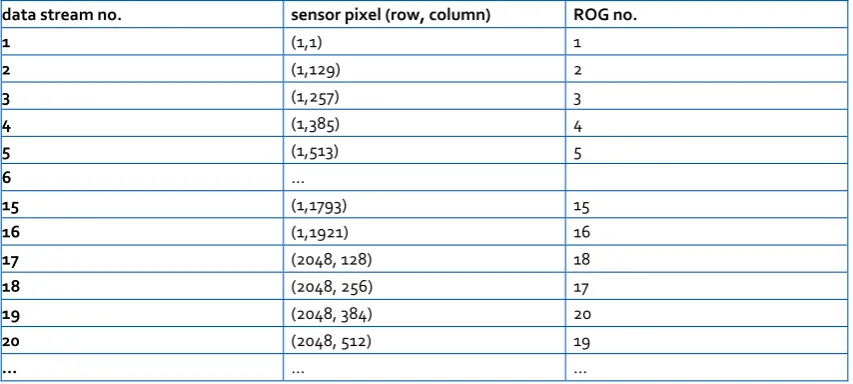
The sensor is divided into an upper and a lower part. Both sections are electrically separated. The data of each section is transferred by 32 “read out groups” (ROG). Each ROG has 128 channels for the detector. The upper groups scan the sensor columns from left to right. The lower groups scan from right to left. The upper groups are transferred first, followed by the lower groups. The upper groups start read out from the upper row. The lower groups start read out from the last row.

The following Table 20 displays the data stream forXRD 1621:

data stream no. sensor pixel (row, column) ROG no.

1 (1,1) 1

2 (1,129) 2

3 (1,257) 3

4 (1,385) 4

5 (1,513) 5

6 …

15 (1,1793) 15

16 (1,1921) 16

17 (2048, 128) 18

18 (2048, 256) 17

19 (2048, 384) 20

20 (2048, 512) 19

… … …

Table 20 Sorting scheme of the XRD 1621

Figure 1: Sorting scheme of the XRD 1621 detector. Each read out group has 128 channels for the detector. The upper groups scan the sensor columns from left to right. The lower groups scan from right to left. The upper groups are transferred first. The upper groups start read out from the upper row. The lower groups start read out from the last row.

In the literature, dysfunctional pixels are referred to by many names including bad, dead, erratic, stuck, hot, defective, broken and underperforming,and a variety of concep-tions is associated with them.

Let n1 and n2 be the number of pixels in the horizontal and the vertical directions,

respectively. An image taken by the detector in a fixed time point is denoted by Z = (Zi)i∈I, where Zi is the value of the pixel i in the grid I = [1, . . . , n2]×[1, . . . , n2]. Let

Z = median{Zi|i ∈ I} be the median of the pixel values across the whole grid and

σ(Z) = SD{Zi|i∈I} be their SD.

For a sequence (Zi(j))i∈I (j = 1, . . . , m) of m such images we define, pixel wise, the median imageand theSD image:

Zi = median{Zi(j)|j= 1, . . . , m} (i∈I), (1)

σ(Z)i = SD{Xi(j)|j = 1, . . . , m} (i∈I). (2)

We define summaries of these images across the whole grid: Z = median{Zi|i∈I} is the median of the median image, σ(Z) = SD{Zi|i∈ I} is the SD of the median image, and

3

The detector manufacturer PerkinElmer performs a final quality test and creates an underperforming pixel mapto be delivered with the detector. They use a number of criteria to classify a pixel asunderperforming based on signal intensities, noise levels, uniformity and lag. We summarise the criteria below and refer to the detector manual [6] for further details.

All tests are accomplished in the Timing 0 (133.2ms; ES: T0 = 66.6ms), 200µm and at

1pF capacity, unless otherwise indicated. The bright image has a nominal value of roughly 30,000 units.

Signal sensitivity: Three types of underperforming pixels are detected through unusual

response in a bright offset corrected image at three different X-ray energies at first free running timing.

• Underperforming bright pixel: value is greater than 150% of the median bright • No gain pixel: dark pixel with no light response

• Underperforming dark pixel: value is below 45% of the median bright

Bright noise: A sequence (Xi(j))i∈I(j= 1, . . . , m) ofm= 100 bright images in the first

free running timingT0 is acquired. Pixeliis called underperforming bright noise pixel if

σ(Z)i>6σ.

Dark noise: A sequence (Zi(j))i∈I(j = 1, . . . , m) of m = 100 dark images in two free

running timingsT0 and T1 is acquired. Pixel iis called underperforming dark noise pixel

ifσ(Z)i>6σ.

Uniformity: These criteria address maximum allowed deviations from overall means and

from nearest neighbours. Let (Zi)i∈I be an image acquired at T0, corrected with gain?

and offset? images also acquired atT0.Pixel i is calledunderperforming (with respect to

global uniformity),if

Zi/Z >1.02 OR Zi/Z <0.98. (3)

Pixeliis called underperforming (with respect to local uniformity),if

Zi/Xi3×3 >1.01 OR Zi/Zi3×3 <0.99. (4)

Lag: The detector is set to an integration time of 2s (triggered mode). Three offset corrected frames are acquired: ImageZ(1) is irradiated during the gap after the readout time of the detector of up to 30,000units, and Z(2) and Z(3) are the following two dark images (first frame after exposure and second frame after exposure). A pixel iis marked asunderperforming,if

Z_i(2)/Z_i(1) > α1 OR Z_i(3)/Z_i(1)> α2 (5)

with thresholdsα1 = 0.08 andα1 = 0.04 in the standard option (orα1= 0.1 andα1= 0.05

in the CsI option).

1. mean white image containing the pixel wise means of the intensities of 100 white acquisitions, as well as images of the corresponding SDs, minima and maxima,

2. mean black image containing the pixel wise means of the intensities of 100 black acquisitions, as well as images of the corresponding SDs, minima and maxima,

3. a mean grey image containing the pixel wise means of the intensities of 100 images acquisitions (standard deviations, minima and maxima arenotincluded),

4. list of bad pixel locations stored in an.xlm file.

Bad pixel maps in X-ray machines are routinely taken after a new detector is installed or an old one is reinstalled after refurbishment. Operators also have the option to take them at times of their convenience. In practice, they usually do so if they feel there “may be something wrong” with the detector.

The data set analysed in this paper comes from a collection of ten bad pixel maps taken between June 2013 and January 2014 on a X-ray machine with a PerkinElmer digital X-Ray Detector XRD 1621 AN/CN by the Warwick Manufacturing Group. Our analysis is based on the first six acquisitions, because the last four contain binned pixels, which implies that some of the information is lost making them less interesting for the analysis. The detector was refurbished between the fourth and the fifth acquisition. For more details see Figure 2.

Preliminary data set

Total of 100 images that contain some information

10 bad pixel maps, regular and binned

Image dimensions and dates

Timestamp WhiteX WhiteY GreyX GreyY BlackX BlackY A_0 2013-06-13 13.31.51 2000 2000 2000 2000 2000 2000 B_0 2013-07-01 11.49.29 2000 2000 2000 2000 2000 2000 C_0 2013-10-02 13.41.00 1600 2000 1600 2000 1600 2000 E_0 2013-11-22 10.54.30 1600 2000 1600 2000 1600 2000 F_0 2014-01-28 11.48.00 2000 2000 2000 2000 2000 2000 G_0 2014-01-28 15.14.02 2000 2000 2000 2000 2000 2000 A_1 2013-06-13 16.14.34 1000 1000 1000 1000 1000 1000 D_1 2013-10-15 09.29.43 800 1000 800 1000 800 1000 F_1 2014-01-28 11.58.23 1000 1000 1000 1000 1000 1000 G_1 2014-01-28 15.19.30 1000 1000 1000 1000 1000 1000

Figure 2: Bad pixel maps. Test data collected by Warwick Manufacturing Group 2013-14 including acquisition date and x and y coordinate dimensions for each of the three parts: white image, grey image and black image. The last four of them contain binned images, that is, pixels are merged in pairs resulting in smaller images. The dimensions vary as a result of the binning and also because the images were cropped after an excess of bad pixels was detected near the edges.

3

Exploratory data analysis of bad pixel maps

5

Local defects: Dead lines

Lines on bad pixel images

Also visible on white, grey and sometimes black images

Going from centre vertical line outwards

A_0: White image

Figure 3: Lines between clusters and midline. Left part of grey image of A 0 shown after 90 degree anticlockwise rotation. Horizontal midline (shown here as vertical line) divides upper row (shown on the left) from lower row (shown on the right). It shows parallel lines connected to the midline from both sides. There is also visible inhomogeneity of intensity, with darker areas near the corners.

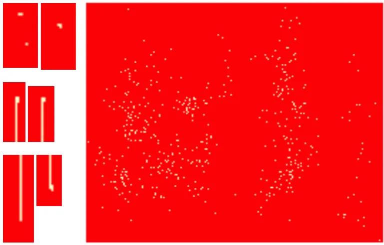
Our systematic assessment of the spatial locations of bad pixels is based on bad pixel lists. Our tool for this are bad pixel images, that is, an image created from the list of bad pixel coordinates (stored in an .xml file as part of the bad pixel map, see Section 2 for details) as coloured squares in their original location in a grid. As colour code we use beige for bad pixels and red for others. (Printed in grey scale, the bad pixels are displayed as bright on a dark background.)

3.1 A taxonomy for bad pixel arrangements

Visual inspection of all the bad pixel images in our data set revealed several types of spatial arrangements of bad pixels. We have classified them into six categories listed below. Nearest neighbourof a pixel refers to the pixels on the left, right, top or bottom of the pixel; the pixels touching it only at corners (diagonal) are not included. A corner piececonsists of three neighbouring pixels that are not in a line.

1. Singletons. Individual bad pixels.

2. Doubles. Two neighbouring bad pixels.

3. Small clusters. Three or more neighbouring bad pixels including at least one corner piece.

4. Lines to midline. Three or more bad pixels arranged in a line leading up to the midline that divides the upper from the lower row of subpannels.

5. High density regions. Areas with visibly higher concentration of single bad pixels.

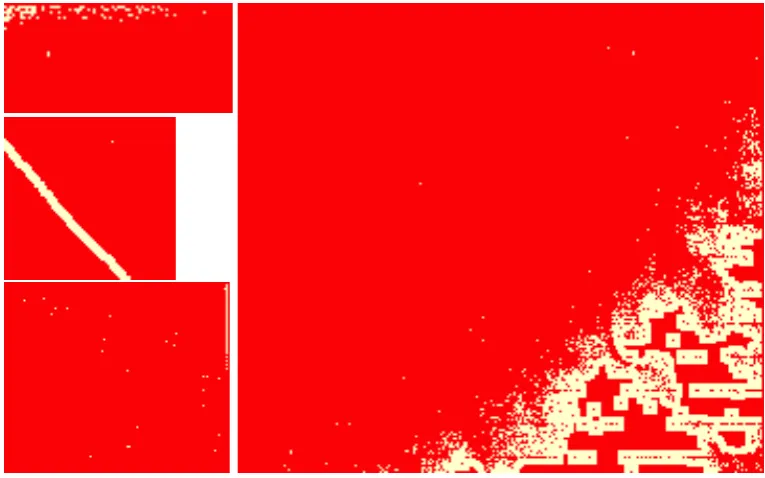
6. Corner damage. Massively damaged area in a corner amounting to connected areas of damage as shown in Figure 5.

clusters and lines occur together. However, there are instances of lines of bad pixels that are connected to the midline on one end, but do that do not end in a cluster on the other end (bottom left in Figure 4), and there are also instances of small clusters that are not connected to a line. Figure 5 shows the four corner areas of the bad pixel image for B 0, all heavily damaged.

Figure 4: Spatial arrangements of bad pixels. Selected areas from bad pixel images A 0 to F 0. The two areas in the upper left row shows singletons, doubles and corner pieces. Three of the other four areas on the left show small clusters with consequent lines as well as one line with no cluster. The big area on the right is a region of high density of bad pixels.

The black and white plots in Figure 6 show the locations of bad pixels for the six regular bad pixel maps in our data set (not the binned ones). There are many dysfunctional lines going up and down from the midline in the first four images. After that, the detector was refurbished and the last two images demonstrate that most of the lines have now disappeared. However, both of these images have areas with high bad pixel intensity that were not present in previous images.

3.2 A closer look on dysfunctional lines

The acquisitions that produced the largest number of lines are C 0 and E 0 with 9 dys-functional lines in the upper row of subpanels and 8 lines in the lower row. A 0 has 7 and 5 and B 0 has 7 and 8, usually in the same locations as C 0 and E 0, though length may vary. F 0 and G 0 were obtained after refurbishment of the panel and only have one line in the upper row and one line in the lower row.

7

Local defects: Corners

Figure 5: Corner damage. Corner areas of bad pixel images for B 0. All four corner areas are seriously damaged.

horizontal midline. The exception is a line in column 744 in F 0, which ends 4 pixels before it reaches the midline. For the other end there are three possibilities: ending in just one pixel, running all the way to the other side of the sub panel, or ending somewhere in a small cluster. The last two options are the most frequent ones. The clusters have some commonalities. Broadly speaking they are 1 to 3 doubled up bad pixels to the right of the line. To illustrate this in more detail, here is a list of the types of all the 17 non-midline ends in C 0 with their frequency

1. line ends in one pixel somewhere in the sub panel: 1

2. line runs to the other side of the sub panel: 4

3. line ends in a small cluster: 12, of which

• endpoint of the line has another bad pixel adjacent to it on the right: 7 • last two pixels of the line have bad pixels adjacent to it on the right: 4 (in one

case there is an extra bad pixel to the left, too)

• last three pixels of the line have bad pixels adjacent to it on the right: 1 (on top of that, there is an extra bad pixel above these adjacent pixels)

9

www.ls.eso.org/lasilla/Telescopes/3p6/efosc/docs/BADPIXMASK/Ccd40Cosmetics.html,

www.astro-wise.org/portal/howtos/man_howto_hot/man_howto_hot.shtml.

It has been suggested that dysfunctional pixels destroy the value of all pixels behind the broken pixel as charge is moved through it during the read-out process. In the analysis of the lines, we will therefore focus on the locations and shapes of the endpoints rather than the modelling the occurrence of complete lines.

4

Spatial models and analysis

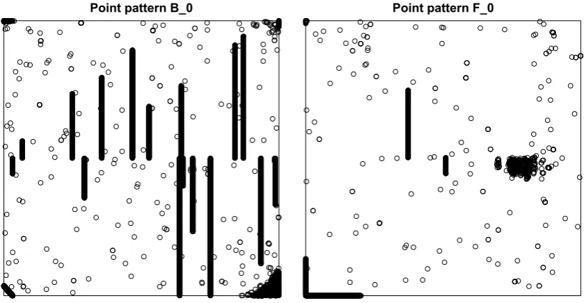
Our models for the spatial distribution of dysfunctional pixels is based on random point patterns. An overview of these models and methods can be found, for example, in [5] and [1], with the latter emphasising on R-implementation using packages such asspatstat, sp and dependencies. Once the data has been imported into a ppp-object, it is straight forward to plot images of the point pattern highlighting the events by out-of-scale plotting characters. Figure 7 shows such images of the detector before and after refurbishment.

Point pattern B_0 Point pattern F_0

Figure 7: Point patterns. B 0 and F 0 straight from raw data showing the difference before and after refurbishment.

There are two perspectives leading to different mathematical descriptions of the de-tector and its dysfunctional pixels. In the previous sections, we recorded the state of the detector at one moment in time as a random field indexed by the two-dimensional grid

I = [1, . . . , n2]×[1, . . . , n2]. The values of the random field can be numeric to describe

the actual value of the pixel or they can be binary indicating its dysfunctional versus functional status. The latter can also be extended to taking categorical values accounting for different types of dysfunctionality.

spatial point processXwith valuesxkin the rectangleS = [0, n2]×[0, n2],with finite total

intensity. Points correspond to the event that the pixel centred there is dysfunctional. For any A ⊆S, the number of points in A is denoted by N(A), and N = N(S) is the total number of points.

To build appropriate spatial point pattern models we briefly return to our taxonomy of damages from Section 3. We first exclude two of the damage types from modelling.

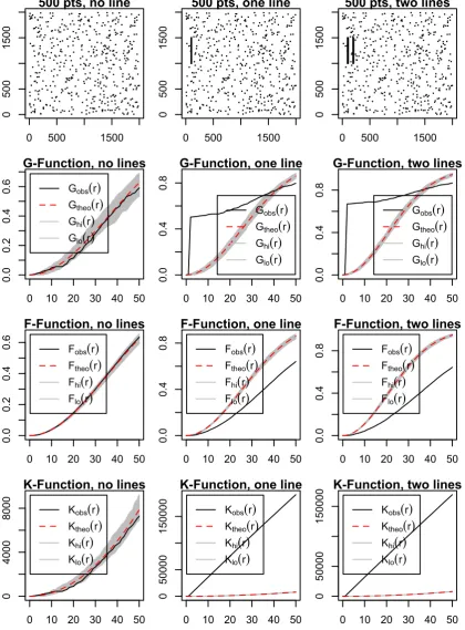
Firstly, we do not include the whole dysfunctional lines, but restrict ourselves to mod-elling the small clusters at the end far off the midline. (In the rare case where there is no cluster, we only use the endpoint.) This is necessary, because even very few short lines quickly dominate calculations testing for CSR making it impossible to detect what goes on in the rest of the image. This is illustrated by simulations in Figure 9, using the descriptive functional statistics known as G-, F-, and K-functions, described for example in [3]. The simulations show how sensitively these react to even just one or two short lines for point densities slightly higher than in our images. The effect on G and K is particularly sharp with obvious changes inr = 1 caused by the sudden huge increase in the number of adjacent bad pixels. It gets more pronounced for lower densities and less pronounced for higher densities; see Figures 14 and 15 in the appendix.

Secondly, the corner damages are rather peculiar and not well suitable for modelling. Since they are located at the margins of the images, restricting models to a cropped image is an appropriate strategy and reflects the common practice of reducing the FOV of the detectors after issue have been detected near the edges. C 0 and E 0 were already cropped by 200 rows both on top and bottom during acquisition. Based on visual inspection we cropped an additional 50 rows on these and accordingly cropped A 0 and B 0 by 250 rows both on top and bottom. The images acquired after refurbishment of the projector, F 0 and G 0, were cropped by 5 pixels all around to exclude artefacts on the edges. Figure 8 shows the point patterns after removal of lines and illustrates the relevance for cropping.

We now study fundamental properties of the spatial point patterns including complete spatial randomness (CSR), homogeneity and intensity estimation as described for example in [3].

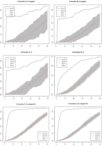
The G-, F-, and K-Functions for our data have been calculated based on 100 Monte Carlo simulations under CSR. Default confidence intervals of 96% are used. For each of the images, the G-Function in Figure 10 indicates aggregation for short ranges, while they seem to behave more randomly at larger distances. A 0, B 0 and C 0 show a jump like increase inr = 1,but little further increase beyond. In contrast, E 0, F 0 and G 0 increase about equally strongly, but more smoothly for small r. This is most likely related to the existence of a small area of high density of bad pixels in the last three images, but not the first three. In turn, the deviations from CSR in the first three images are the result of an unusually high amount of doubles and very small clusters (see last column in Table 13). The behaviour of the F-Functions in Figure 11 confirms this, with aggregation particularly pronounced in the last two images.

11

Point pattern w/o lines A_0 Point pattern w/o lines B_0

Point pattern w/o lines C_0 Point pattern w/o lines E_0

Point pattern w/o lines F_0 Point pattern w/o lines G_0

0 500 1500

0

500

1500

500 pts, no line

x

0 10 20 30 40 50

0.0

0.2

0.4

0.6

G-Function, no lines

r

Gobs(r

)

Gtheo

(

)

(

)

Glo

(

)

0 10 20 30 40 50

0.0

0.2

0.4

0.6

F-Function, no lines

r

Fobs(r

)

Ftheo

(

)

(

)

Flo

(

)

0 10 20 30 40 50

0

4000

8000

K-Function, no lines

Kobs(r

)

Ktheo

(

)

(

)

Klo

(

)

0 500 1500

0

500

1500

500 pts, one line

x

y

0 10 20 30 40 50

0.0

0.4

0.8

G-Function, one line

r

G

(

r

)

)

Gtheo

(

)

(

)

Glo

(

)

0 10 20 30 40 50

0.0

0.4

0.8

F-Function, one line

r

F

(

r

)

Fobs(r

)

Ftheo

(

)

(

)

Flo

(

)

0 10 20 30 40 50

0

50000

150000

K-Function, one line

K

(

r

)

Kobs(r

)

Ktheo

(

)

(

)

Klo

(

)

0 500 1500

0

500

1500

500 pts, two lines

x

y

0 10 20 30 40 50

0.0

0.4

0.8

G-Function, two lines

r

G

(

r

)

)

Gtheo

(

)

(

)

Glo

(

)

0 10 20 30 40 50

0.0

0.4

0.8

F-Function, two lines

r

F

(

r

)

Fobs(r

)

Ftheo

(

)

(

)

Flo

(

)

0 10 20 30 40 50

0

50000

150000

K-Function, two lines

K

(

r

)

Kobs(r

)

Ktheo

(

)

(

)

Klo

(

)

13

0 10 20 30 40 50

0.0

0.2

0.4

0.6

0.8

G function G_0 cropped (5)

r

G

(

r

)

Gobs(r) Gtheo(r)

Ghi(r)

Glo(r)

0 10 20 30 40 50

0.0

0.2

0.4

0.6

0.8

G function E_0

r

G

(

r)

Gobs(r) Gtheo(r) Ghi(r)

Glo(r)

0 10 20 30 40 50

0.0 0.1 0.2 0.3 0.4 0.5

G function B_0 cropped

r

G

(

r

)

Gobs(r) Gtheo(r) Ghi(r)

Glo(r)

0 10 20 30 40 50

0.0 0.1 0.2 0.3 0.4 0.5

G function C_0

r

G

(

r

)

Gobs(r) Gtheo(r) Ghi(r)

Glo(r)

0 10 20 30 40 50

0.0

0.1

0.2

0.3

0.4

G function A_0 cropped

r

G

(

r

)

Gobs(r) Gtheo(r)

Ghi(r)

Glo(r)

0 10 20 30 40 50

0.0

0.2

0.4

0.6

0.8

G function F_0 cropped (5)

r

G

(

r

)

Gobs(r) Gtheo(r)

Ghi(r)

Glo(r)

0 10 20 30 40 50 0.0 0.1 0.2 0.3 0.4

F function B_0 cropped

r

F

(

r

)

Fobs(r)

Ftheo(r) Fhi(r) Flo(r)

0 10 20 30 40 50

0.0

0.2

0.4

0.6

0.8

F function G_0 cropped (5)

r

F

(

r

)

Fobs(r)

Ftheo(r) Fhi(r) Flo(r)

0 10 20 30 40 50

0.0

0.1

0.2

0.3

0.4

F function E_0

r

F

(

r)

Fobs(r)

Ftheo(r) Fhi(r) Flo(r)

0 10 20 30 40 50

0.00 0.05 0.10 0.15 0.20 0.25 0.30

F function A_0 cropped

r

F

(

r

)

Fobs(r)

Ftheo(r) Fhi(r) Flo(r)

0 10 20 30 40 50

0.0

0.1

0.2

0.3

0.4

F function C_0

r

F

(

r)

Fobs(r)

Ftheo(r) Fhi(r) Flo(r)

0 10 20 30 40 50

0.0

0.2

0.4

0.6

0.8

F function F_0 cropped (5)

r

F

(

r

)

Fobs(r)

Ftheo(r) Fhi(r) Flo(r)

15

0 50 100 150 200

-1 50 00 -1 00 00 -5 00 0 0 5000 10000 15000 20000

K function normed A_0 cropped

r K ( r ) − π r 2

Kobs(r)−πr2 Ktheo(r)−πr2 Khi(r)−πr2 Klo(r)−πr2

0 50 100 150 200

-1 00 00 -5 00 0 0 5000 10000 15000

K function normed B_0 cropped

r K ( r ) − π r 2

Kobs(r)−πr2 Ktheo(r)−πr2 Khi(r)−πr2 Klo(r)−πr2

0 50 100 150 200

-1 00 00 0 10000 20000 30000

K function normed C_0 cropped

r K ( r ) − π r 2

Kobs(r)−πr2 Ktheo(r)−πr2 Khi(r)−πr2 Klo(r)−πr2

0 50 100 150 200

0e +0 0 1e +0 5 2e +0 5 3e +0 5 4e +0 5

K function normed E_0 cropped

r K ( r ) − π r 2

Kobs(r)−πr2 Ktheo(r)−πr2 Khi(r)−πr2 Klo(r)−πr2

0 50 100 150 200

0e +0 0 2e +0 5 4e +0 5 6e +0 5 8e +0 5 1e +0 6

K function normed F_0 cropped

r K ( r ) − π r 2

Kobs(r)−πr2 Ktheo(r)−πr2 Khi(r)−πr2 Klo(r)−πr2

0 50 100 150 200

0 50000 100000 150000 200000 250000 300000

K function normed G_0 cropped

r K ( r ) − π r 2

Kobs(r)−πr2 Ktheo(r)−πr2 Khi(r)−πr2 Klo(r)−πr2

are additional small range interactions from the areas with increased density of bad pixels (see Figure 8).

The observed intensities are summarised in Table 13. The assumption of homogeneity seems suitable for the first four images (after suitable cropping of corners and edges). For the last two images a homogeneity assumption seems wrong, given each of them has a quite well defined area with an strongly increased density of bad pixels. The obvious alternative is to consider inhomogeneous models. However, the areas of high intensity of bad pixels may be the result of somewhat arbitrary cut-offs in the definition of bad pixels. A sensitivity analysis based on varying these cut-offs is recommended.

Areas Number of _{bad pixels} Intensities _{in selected area}Small clusters

A_0 _{[0,2000]x[250,1750]}[0,2000]x[0,2000] 625₁₂₇ 15.625 _{4.233 16 [12.6%]}NA

B_0 _{[0,2000]x[250,1750]} [0,2000]x[0,2000] 7053 ₁₇₅ 176.325 _{5.833 26 [14.9%]}NA

C_0 _{[0,2000]x[250,1750]}[0,2000]x[0,1600] 219₁₈₀ 6.843 _{6.000 25 [13.9%]}NA

E_0 _{[0,2000]x[250,1750]}[0,2000]x[0,1600] 427₃₆₂ 13.344 _{12.067 21 [ 5.8%]}NA

F_0 [0,2000]x[0,2000]_{[5,1995]x[5,1995]} 1412 ₆₉₄ 35.300 _{17.437 31 [ 4.5%]}NA

G_0 [0,2000]x[0,2000]

[5,1995]x[5,1995]

576

352 14.400 8.844 31 [ 8.8%]NA

Figure 13: Bad pixel counts and intensities. For each image, bad pixel counts for both original image and suitably cropped image (as explained above) are given and corre-sponding intensities (multiplied with the factor 100,000) under homogeneity assumption. The last column shows the number of doubles. (For E 0 and G 0 the counts of doubles exclude the areas of high intensity of bad pixels.

5

Applications to detector performance monitoring

Based on the models introduced in the last section we suggest the following basic protocol for detector performance monitoring. The emphasis of the protocol is on the spatial distribution of dysfunctional pixels. This protocol can be used to establish benchmarks for detector performance, more specifically, for objectives including the following:

• Determining sufficiently functional FOV; • Determining need for refurbishment;

17

• Detecting performance differences between subpanels;

• Linking defects to problems in the detector manufacturing process or usage.

The protocol can be carried out employing some of the diagnostic tools used in the previous sections. The starting point for the analysis is the list of bad pixel locations.

1. View. Visualise the location of the bad pixels by plotting them in their original

locations in a square. Diagnostic tools: Plots as in Figure 7 give a quick impression.

2. Classify. Make a frequency table of all types of spatial arrangements of bad pixels

in the data set. This is to confirm whether the panel has the types of defects known from previously studied panels and potentially adds new types to the list. Diagnostic tools: Plots as in Figure 6 are suited to view details. It may be necessary to zoom in, because individual pixels are very small.

3. Crop. Based on visual inspection using the plots from the first two steps, reduce

image by cropping marginal rows and/or columns as appropriate, to exclude corner or edge issues currently not addressed by modelling.

4. Model. Fit a spatial point pattern model.

(a) If lines occur in the bad pixel map image, keep only the endpoint far the middle line in the bad pixel list.

(b) Examine whether the remaining pattern is random in the sense of complete spatial randomness (CSR). If it is not random, determine whether there may be regularity or aggregation. Determine which point distances drive these be-haviours. Diagnostic tools: Study the graphs of the G-, F- and K-Functions, as shown in Figures 10, 11 and 12.

(c) Estimate the intensity under homogeneity assumptions, as appropriate. Oth-erwise consider fitting a heterogeneous density. However, since the definition of bad pixel is based on thresholds and the scanning has been performed under not necessarily universal parameters, back this up with sensitivity analysis.

5. Subpanels. Perform the model fit sketched above separately for the different

sub-panels. Check whether there are systematic differences between the subpanel that could potentially be linked to the manufacturing process or modes of usage. Diag-nostic tools: As in previous steps. In addition, plot of the bad pixel locations on the panel can be overlaid with a grid showing the subpanel division for visual examina-tion of subpanel related artefact. A χ2-test for independence can be performed on the counts of bad pixels on the subpanels.

6

Discussion, conclusions and future work

their spatial arrangements: Singletons, doubles, small clusters, high density patches, lines and corner damage.

The last two types of damages are treated differently than the others. Corner damages are related to known physical causes such as increased stress related to mounting and more rigidity of the material closer to the corners. The damage caused by them can be controlled by adjusting the FOV of the detector. We therefore exclude corner damages from the modelling. Dysfunctional lines can start in any location and, with the notable exception of one in this data set, end at the midline. The most common explanation is that they are the result of a data stream interruption due to a single or, more typically, small cluster of bad pixels on one end. We therefore restrict the spatial analysis to the non-midline endpoints of the dead lines.

The occurrence of singletons, doubles and small clusters of bad pixels has been studied using models for spatial point patterns. Using G-, F- and K-functions, we found that all the six images deviate from the CSR assumption due to aggregation on small ranges, even very ones. There are two obvious potential reasons for these deviation, and it is likely that what remains after their removal would actually fulfil the CSR assumptions.

The first reason are small areas of high density as found in E 0, F 0 and G 0. They could be excluded from the model like the corners. Or they could be modelled using non-homogeneous processes. However, they typically have quite clear boundaries potentially leading to an intensity function with high gradients.

The second reason are unusually high numbers of doubles and very small clusters that are not matched by comparable aggregation at bigger ranges. The unexpected frequency of doubles and small clusters was one of the bigger surprises in this data analysis. Asking for the reason brings us back to the original set-up of the spatial point pattern model. In our models, we have identified points with the event that an individual grid pixel is dysfunctional. It can be argued, though, that the elementary event of interest is a kind of damage that can extend to one, two or a small cluster of pixels as part of the same mathematical event. This is a very intuitive approach for the scenario where damage is caused by an external force that may hit the panel in a small location covering some amount of pixels up to a small cluster. Hence, an alternative set-up for the spatial point process models would be to identify points with dysfunctional locations of the size up to small clusters counting them as one only.

Translating this intuition into a formal model has to overcome two hurdles. Firstly, the definition of what a small cluster is, as opposed to say several adjacent clusters or a small region of high density, will remain somewhat arbitrary. Secondly, clusters may contain pixels with different types of dysfunctionality, making it complicated to assign a mark for the points representing these events.

Furthermore, our perspective is blind to the original arrangement of the pixels in a grid. There, the vertical and the horizontal direction are distinguished, reflecting the physical structure of the panel. Another investigation would be to pay special attention to the behaviour along both of these directions. In other words, the spatial point process perspective could be supplemented by one-dimensional analysis.

19

to create the bad pixel map. The more characteristic damages at the corners and edges, and the isolated singleton, doubles and small clusters, may persist independent of these settings. However, it has been suggested by users that some of the patches with high bad pixels density are sensitive to these settings.

We have focused on spatial arrangement of pixels classified as bad according to the bad pixel map protocol of the kind used byNikon. Future work should extend the current discussing including also the temporal evolution of pixel dysfunctionality. A collection of test images taken at regular intervals over an extended period of time should be assembled. An initial step of temporal modelling includes determining potential stages until a pixel is fullydead, analyse how long pixels typically stay in these stages and find out whether they can move between them. Combining this with results from spatial analysis, spatio-temporal models for pixel damage should be fitted.

In terms of the models used, different types of dysfunctionality can be accounted for by extending this set-up to a marked spatial point process. For example, marks could be assigned to distinguish ends of lines from isolated small damages, or to label pixels according to different criteria for underperformance listed in Section 2.

The methods presented here have practical applications to the monitoring, refurbish-ment and manufacturing of detectors. A toolbox of statistical techniques is presented and can be put to use as needed by users of the detectors. For example, comparing the dam-age intensity across subpanels determines whether some of them need to be exchanged. Spatial patterns of bad pixels may give clues to the causes of the damage related to either the manufacturing or the time or modes of use.

Acknowledgements

The authors wish to acknowledge funding by EPSRC grant EP/K031066/1.

References

[1] Roger S Bivand, Edzer J Pebesma, and Virgilio G´omez-Rubio. Applied spatial data analysis with R, volume 747248717. Springer, 2008.

[2] Angela Cantatore and Pavel M¨uller. Introduction to computed tomography. Technical report, DTU Mechanical Engineering, 2011.

[3] Sung Nok Chiu, Dietrich Stoyan, Wilfrid Stephen Kendall, and Joseph Mecke. Stochas-tic Geometry and Its Applications. John Wiley and Sons, June 2013.

[4] Maire E. and Withers P. J. Quantitative X-ray tomography. International Materials Reviews, 59(1):1–43, 2013.

[5] Carlo Gaetan, Xavier Guyon, and Kevin Bleakley. Spatial statistics and modeling, volume 271. Springer, 2010.

7

Appendix

0 500 1500

0

500

1500

100 pts, no line

x

0 10 20 30 40 50

0.00

0.10

0.20

0.30

G-Function, no lines

r

Gobs(r) Gtheo(r)

Ghi(r) Glo(r)

0 10 20 30 40 50

0.00

0.10

0.20

F-Function, no lines

r

Fobs(r)

Ftheo(r)

Fhi(r)

Flo(r)

0 10 20 30 40 50

0

4000

8000

K-Function, no lines

Kobs(r)

Ktheo(r)

Khi(r)

Klo(r)

0 500 1500

0

500

1500

100 pts, one line

x

y

0 10 20 30 40 50

0.0

0.4

0.8

G-Function, one line

r

G

(

r

) Gobs(r)

Gtheo(r)

Ghi(r) Glo(r)

0 10 20 30 40 50

0.0

0.2

0.4

0.6

F-Function, one line

r

F

(

r

)

Fobs(r)

Ftheo(r)

Fhi(r)

Flo(r)

0 10 20 30 40 50

0e +0 0 2e +0 5 4e +0 5

K-Function, one line

K

(

r

)

Kobs(r)

Ktheo(r)

Khi(r)

Klo(r)

0 500 1500

0

500

1500

100 pts, two lines

x

y

0 10 20 30 40 50

0.0

0.4

0.8

G-Function, two lines

r

G

(

r

) Gobs(r)

Gtheo(r)

Ghi(r) Glo(r)

0 10 20 30 40 50

0.0

0.4

0.8

F-Function, two lines

r

F

(

r

)

Fobs(r)

Ftheo(r)

Fhi(r)

Flo(r)

0 10 20 30 40 50

0

100000

250000

K-Function, two lines

K

(

r

)

Kobs(r)

Ktheo(r)

Khi(r)

Klo(r)

Figure 14: Sensitivity to lines. Simulations of random scatters of 100 points (low intensity) on a 2000 x 2000 grid with no, one or two lines of length 500 added to it. The G-, F-, and K-Function estimates are calculated based on 49 CSR simulations. Scales on

21

0 500 1500

0

500

1500

1000 pts, no line

x

0 10 20 30 40 50

0.0

0.4

0.8

G-Function, no lines

r

Gobs(r) Gtheo(r)

Ghi(r) Glo(r)

0 10 20 30 40 50

0.0

0.4

0.8

F-Function, no lines

r

Fobs(r)

Ftheo(r)

Fhi(r)

Flo(r)

0 10 20 30 40 50

0

2000

6000

K-Function, no lines

Kobs(r)

Ktheo(r)

Khi(r)

Klo(r)

0 500 1500

0

500

1500

1000 pts, one line

x

y

0 10 20 30 40 50

0.0

0.4

0.8

G-Function, one line

r

G

(

r

) Gobs(r)

Gtheo(r)

Ghi(r) Glo(r)

0 10 20 30 40 50

0.0

0.4

0.8

F-Function, one line

r

F

(

r

)

Fobs(r)

Ftheo(r)

Fhi(r)

Flo(r)

0 10 20 30 40 50

0

40000

80000

K-Function, one line

K

(

r

)

Kobs(r)

Ktheo(r)

Khi(r)

Klo(r)

0 500 1500

0

500

1500

1000 pts, two lines

x

y

0 10 20 30 40 50

0.0

0.4

0.8

G-Function, two lines

r

G

(

r

) Gobs(r)

Gtheo(r)

Ghi(r) Glo(r)

0 10 20 30 40 50

0.0

0.4

0.8

F-Function, two lines

r

F

(

r

) Fobs(r)

Ftheo(r)

Fhi(r)

Flo(r)

0 10 20 30 40 50

0e +0 0 4e +0 4 8e +0 4

K-Function, two lines

K

(

r

)

Kobs(r)

Ktheo(r)

Khi(r)

Klo(r)

Figure 15: Sensitivity to lines. Simulations of random scatters of 1000 points (high intensity) on a 2000 x 2000 grid with no, one or two lines of length 500 added to it. The G-, F-, and K-Function estimates are calculated based on 39 CSR simulations. Scales on