University of Warwick institutional repository: http://go.warwick.ac.uk/wrap
A Thesis Submitted for the Degree of PhD at the University of Warwick
http://go.warwick.ac.uk/wrap/77466
This thesis is made available online and is protected by original copyright. Please scroll down to view the document itself.
Essays on practical issues in asset
pricing: estimation and simulation
Thesis
Submitted to the University of Warwick
for the degree of
Doctor of Philosophy
by
YAN WANG
supervised by
Dr. Xing Jin
Acknowledgment
A large number of people contributed directly and indirectly to the accomplishment of
this thesis. Most of all, I want to thank my supervisor Dr. Xing Jin. He introduced me
to the subject of my research and gave me the opportunity that conducted to this thesis.
His support and contagious enthusiasm were absolutely essential for me. I also thank Dr.
Nick Webber who provided full support and drew me to this area at the very beginning.
I would like to thank both the University of Warwick and Warwick Business School, who
supported me both financially and academically. I want to thank Kevin, for the support
he has shown during the past many years. I could not have finalized this thesis without
him.
At last, a special thanks goes to my new friends at the University of Warwick and those
old yet lifetime ones spread over the world, who always encouraged me, helped me in dark
Declarations
The work submitted in this thesis is the result of my own investigation, except where
otherwise stated. It has not already been accepted for any degree at another university,
Contents
Acknowledgment ii
Declarations iii
List of Figures vii
List of Tables ix
Abstract xi
1 General Introduction 1
2 An empirical study on MCMC estimation for return dynamics with
time-changed L´evy processes 6
2.1 Introduction . . . 6
2.2 MCMC estimation and L´evy type models . . . 12
2.2.1 Markov Chain Monte Carlo estimation . . . 12
2.2.2 L´evy processes and L´evy type models . . . 15
2.3 An empirical study of time-changed L´evy processes with MCMC . . . 25
2.4 Empirical results of time-changed L´evy processes . . . 29
2.5 Conclusion . . . 39
3 An Empirical Study of Multivariate MCMC Estimation on L´evy pro-cesses 41 3.1 L´evy Model Specification . . . 45
3.1.1 The Normal inverse Gaussian process (NIG) . . . 49
3.1.2 The Merton jump-diffusion process (MJD) . . . 50
3.2 Model Estimation . . . 51
3.2.1 Data Augmentation . . . 52
3.2.2 Prior Distributions . . . 53
3.2.3 Complete-Data Likelihood Function . . . 54
3.2.4 Proposal Distributions . . . 54
3.2.5 Choosing the Prior . . . 54
3.3 Empirical Results . . . 56
3.3.1 Estimation assessment . . . 57
3.3.2 Estimating multivariate stochastic dynamics . . . 64
3.4 Conclusion . . . 67
4 Sampling a special case of the SABR model 69 4.1 Introduction . . . 69
4.2 Sampling the CEV dynamics . . . 72
4.2.1 Properties of the CEV dynamics . . . 73
4.2.3 Numerical experiments . . . 79
4.3 Sampling the time-change At. . . 83
4.3.1 The implicit solution of At . . . 84
4.3.2 A numerically indistinguishable alternative, A∗ t . . . 85
4.3.3 Sampling A∗ T . . . 86
4.4 A new representation of the SABR model . . . 90
4.5 Numerical experiments . . . 92
4.6 Conclusion . . . 97
5 General conclusions, contributions and further research 98 Bibliography 101 Appendix A 105 A.1 Detailed description of MCMC algorithm . . . 105
A.1.1 Prior distributions . . . 105
A.1.2 Posterior distributions . . . 106
A.2 Sampling the LS distribution . . . 109
List of Figures
2.1 Time series plot of the MSCI World Index from 02/05/2001 to 31/12/2012 30
2.2 Time series plot of log returns of the MSCI World Index from 02/05/2001
to 31/12/2012 . . . 31
2.3 Kernel density and QQ plot of the residuals of the HJ model . . . 34
2.4 Kernel density and QQ plot of the residuals of the HVG model . . . 35
2.5 Kernel density and QQ plot of the residuals of the SVVG model . . . 35
2.6 Kernel density and QQ plot of the residuals of the SVLS model . . . 36
2.7 Estimated volatilities of HJ, HVG, SVVG, and SVLS models . . . 38
4.1 Density of Xt, p(t;x, y) (y >0) . . . 75
4.2 Probability of Killing with Changing β . . . 76
4.3 Plots of sampled densities ofXT against true densities, whileβ= 0.1,0.5,0.9, σ= 0.2,0.6,1,X0 = 0.5,T = 1 . . . 81
4.4 Plots of sampled densities of FT, while β = 0.1, σ = 0.2, or β = 0.5, σ= 0.6,X0 = 0.5,T = 1 . . . 82
4.5 Simulated density for A∗ T, while σ0 = 0.5, α = 0.3, T = 1, number of sample pathsN = 105, number of discretization steps M = 200 . . . 87
List of Tables
2.1 Estimation results on simulation data for three models . . . 28
2.2 A summary of statistics of daily log returns of the MSCI World Index . . . 30
2.3 Estimation results of the MSCI World Index . . . 33
2.4 Empirical results of Kolmogorov-Smirnov Test . . . 37
3.1 Common factors: Estimation errors expressed in absolute terms. ( RMSE, Bias, Inefficiency ) . . . 60
3.2 Average results relative to the estimated parameters. Estimation errors expressed in absolute terms. RMSE, Bias, Inefficiency . . . 61
3.3 Average MSE, computation times (measured in seconds) and efficiency gains of the two-step approach to the maximum likelihood method. . . 63
3.4 A statistical description for international indices . . . 64
3.5 The optimal estimates of the index data: MJD model . . . 65
3.6 Comparison of moments for the index data: MJD model . . . 66
4.1 Relation between parameters . . . 73
4.2 Probability of XT killing at 0, X0 = 0.5, T = 1 . . . 80
4.4 Parameter sets used in experiments . . . 93
Abstract
This thesis studies several practical issues in asset pricing, including MCMC estimation of
time-changed L´evy processes, calibration techniques for stochastic volatility models, and a
sampling scheme for the SABR model. First, a MCMC estimation approach is developed
to estimate time-changed L´evy processes. Simulation-based experiments demonstrate
good accuracy of the MCMC approach. An empirical study on its fitness of the return
dynamics is provided, which shows that time-changed L´evy models can achieve excellent
performance in capturing index returns. Second, a further study on MCMC estimation is
applied to multivariate L´evy processes, in order to evaluate the efficiency and accuracy of
the Bayesian technique for high-dimensional portfolio theory. Last, a new representation
of the SABR model is proposed by adopting a coupling approach, based on which, the
uncorrelated SABR is sampled from its density. Numerical experiments are implemented
to compare the sampling scheme with the Euler discretization scheme and examine the
Chapter 1
General Introduction
Modelling the return dynamics of individual stocks and indices is a core concern of
a-cademics and practitioners working on the asset pricing theory. A good pricing model
is essential for portfolio allocation, derivatives pricing and risk modelling and
manage-ment. How to choose and use a proper model is actually the mixed field of estimation,
calibration and simulation. For instance, to price and hedge financial derivatives, the
first move is to calibrate the model with the curvature of current market surface. With
the calibrated model, simulation might be needed to price some exotic derivatives which
cannot be priced explicitly. For the portfolio allocation problem, the underlying model
needs to be estimated with a period of historical data. The optimal portfolio weights will
be calculated according to the estimated model. Clearly, asset pricing models can only
be used after either calibration or estimation.
the development of financial markets. Looking back to the history of finance, every
financial crisis has brought some new features to the market such as the crash of October
1987, the burst of the dot-com bubble in 2000, and the recent financial crisis starting in
2007. Nowadays a pricing model has to be able to capture large-size price and volatility
movements on the market. In addition, the model also needs to be able to account for
well-documented stylized facts such as volatility clustering and fat tails in the return
distribution, and must be capable of modeling the leverage effect, and produce the smile
patterns observed in option data.
Jumps in capturing return dynamics along with diffusion were first introduced in Merton
(1976), in order to model large and rare movements of returns. Stochastic volatility
is another famous market feature that has significant impact on option pricing, which
inspires the development of stochastic volatility models such as the celebrated Heston
model proposed by Heston (1993). However, the development of modelling never stop
as the market keeps exhibiting new features that cannot be captured by existing models.
For instance, neither stochastic volatility models nor jump models can explain the market
data in a quantitative sense. In particular, stochastic volatility models fail to explain
large price drops that occur during a single day since it would require an unrealistically
high volatility level before and after the crash. Models with jumps in returns can explain
large price movements, but fail to explain volatility clustering over time.
Merton (1976) starts using jumps by introducing the compound Poisson jump. A more
distribution, which can provide a variety of non-Gaussian distributions. Nowadays, L´evy
processes have become a popular alternative to diffusion, especially in derivative pricing.
Jump risk that represents the sudden loss in the market cannot be modelled by diffusion
models. Imitating the Black-Scholes model, many Geometric L´evy models have been
proposed, such as the Variance Gamma (VG) model (see Madan et al. (1998)) and the
CGMY model (see Carr et al. (2002)).
Simulation is probably the best way to derive fair prices when no explicit solution can
be obtained. PDE method and lattice method all have limitations such as the curse of
dimensionality. Naive simulation methods like the Euler scheme can generate an good
approximation of the derivative price; however, a biased estimator of prices might cause
significantly large losses. Exact-simulation is introduced in order to avoid pricing biases.
The SABR model has been widely used by practitioners in the financial industry, especially
in the interest rate derivative markets. The popularity of the SABR model might be due
to its fast asymptotic solution to implied volatility. The simulation of the SABR model
is very crucial as no explicit solution exists. The probability of touching boundary is a
big issue for simulating the SABR model. Exact-simulation method for the SABR model
is still an open question, which is of great practical value.
In this thesis, three topics associated with practical issues are discussed. Estimation,
cal-ibration and simulation are the most important practical topics of financial engineering.
In chapter 2, a Bayesian Markov Chain Monte Carlo (MCMC) estimation method is
and jumps. The estimation examples show that the MCMC method is capable of
esti-mating L´evy models with very good accuracy, based on simulation data. We also show
that returns produced by time-changed infinite activity L´evy processes cannot be
mod-elled by existing jump-diffusion models. Empirical results suggest that infinite activity
L´evy processes can outperform jump-diffusion models in capturing the variation of index
returns, even without diffusion.
In chapter 3, we consider multidimensional, continuous-time modelling problem where the
observation process is a diffusion with drift and volatility coefficients being modeled as
continuous-time, finite-state Markov chains with a common state process. For the
econo-metric estimation for drift and volatility of the underlying Markov chain, we develop an
discrete-time Markov chain Monte Carlo (MCMC) sampler and compare these approaches
with maximum likelihood (ML) estimation. For simulated data, MCMC outperforms ML
estimation for all scenarios. Finally, for real market index data, we apply the estimation
approach and obtain fit results.
In chapter 4, we propose a new representation of the SABR model, in which, the SABR
model can be seen as a time-changed CEV dynamics. We derive the implicit form of the
time-change, make a guess of its explicit solution and prove the validity of our guess in the
numerical sense. We then try to sample the SABR model based on its new representation.
We first sample the CEV dynamics directly from its density, then sample the time-change
by approximating its time-T distribution with a lognormal distribution by matching their
the time-change, we sample the non-correlated SABR model, compare the performance
of our sampling scheme with the Euler Monte Carlo scheme, and examine the accuracy
of Hagan’s popular asymptotic formula for the implied Black-Scholes volatility.
Chapter 2
An empirical study on MCMC
estimation for return dynamics with
time-changed L´
evy processes
2.1
Introduction
Modelling returns series is a core issue in asset pricing theory. Many models including
both continuous-time models and discrete-time models have been proposed and assessed
for different purposes. The development of modelling always reflects the evolution of the
market. The market keeps exhibiting new features that existing models cannot fit, and
new models in order to follow the market. For instance, the celebrated Black-Scholes
model is the first quantitative model that has a broad range of applications in asset pricing.
The Black-Scholes model assumes that log returns follow Normal distribution; however,
empirical literature documents that market returns do not exhibit either zero-skewness
or low excess-kurtosis. Moreover, after experiencing several financial crises, practitioners
and the academia started to consider and identify the existence of jumps as rare large
movements of stock prices are not so rare. The booming development of the derivatives
market also brings another issue that needs to be taken into account, which is stochastic
volatility. Practitioners realize that volatility risk plays an essential role in pricing and
hedging, which results in the development of Stochastic Volatility (SV) models.
Evaluating the performance of a pricing model seems to be a straightforward job; however,
it is not always the case. For some simple models, there are many possible estimation
methods that can work, such as the Maximum likelihood estimation (MLE) method,
the filtering method, and Generalized method of moments (GMM). Each method has
its advantages and disadvantages. There is no universal method that works for every
circumstance. Estimating multi-dimensional stochastic processes is always a daunting
task. Calibration has also been used as a special approach of estimation, which is still
debatable now as serious statisticians do not take calibration as an estimation technique.
The key difference is that estimation adopts the historical data sampled in a relatively
long period while calibration is usually done on daily basis.
situation can also be found in the field of calibration. Affine Jump-diffusion (AJD) models
have been popular for a long time, because the Fast Fourier Transform (FFT) method
en-ables it to do the calibration procedure in an acceptable time. Despite the disadvantages,
AJD models still have a variety of application in asset pricing. A powerful estimation
technique can boom the development of models and also provide a way to evaluate and
compare the performance of models. Existing estimation methods such as MLE and
G-MM have difficulty in dealing with high-dimensional processes, which limits the use of
sophisticated multi-dimensional asset pricing models.
L´evy processes have become popular and increasingly useful recently. Many literature
have documented the applications of L´evy processes in various fields such as derivatives
pricing, risk management and credit risk modelling ( see Barndorff-Nielsen (1998), Carr
et al. (2002) and Carr and Wu (2003) ). L´evy processes are closely related to Infinitely
Divisible Distribution (see Sato (1999)). Hence, there are many possible choices for the
innovation distribution, in order to capture some market features such as asymmetric
skewness and high kurtosis. Brownian motion is the cornerstone of stochastic modelling
and only a special case of L´evy processes. Generally speaking, a L´evy process is a c`adl`ag
stochastic process that has independent stationary increments. If we impose a
distribu-tion on the increments, we will have a specific L´evy process. L´evy processes have good
economic intuition and provide good flexibility for modeling return dynamics. Moreover,
L´evy processes introduce jumps into modelling, which can capture large and rare
market.
The development of L´evy models brings many new choices for asset pricing theory. Madan
et al. (1998) propose the Variance Gamma (VG) process which provides an asymmetric
distribution. Carr et al. (2002) discuss the empirical performance of several popular L´evy
processes including VG process and CGMY process, in terms of statistical estimation
and risk-neutral estimation. L´evy processes have not been commonly used to solve the
portfolio allocation problem. One of the main reasons is that it is difficult to estimate
L´evy type models. Li et al. (2008) propose a MCMC method to estimate L´evy processes
and assess the performance of L´evy processes with market data. Kallsen and Muhle-Karbe
(2011) develop a method of moments in order to estimate time-changed L´evy processes.
In this chapter, we extend the MCMC method proposed by Li et al. (2008) to deal with
time-changed L´evy processes and investigate whether time-changed L´evy processes can
be used to model return dynamics.
L´evy processes can be categorized by the property of activity rate. Activity rate describes
the intensity of the appearance of jumps. If the activity is infinite, the corresponding L´evy
is said to be an infinite activity L´evy process. In any finite time interval, there will be
infinitely many jumps for an infinite activity L´evy process. In addition to large and rare
jumps, an infinite L´evy process can capture the behaviour of all sizes of jumps, even
without the diffusion component. Our focus is to estimate time-changed L´evy processes
and investigate whether infinite activity L´evy models, despite their theoretical properties,
In this chapter, we aim to develop a MCMC estimation method for time-changed L´evy
models and assess the goodness of fit based on market data. The main contribution
of this chapter can be understood in three aspects. First, we develop the estimation
method with full details, which can be applied to the whole set of L´evy processes. We
will demonstrate whether the MCMC method can jointly estimate both model parameters
and latent variables, especially those small infinite activity jumps. The empirical results
suggest that MCMC estimation can provide very accurate joint identification of L´evy
jumps and stochastic volatility. we demonstrate the accuracy and stability of the MCMC
method based on simulation data. This enables us to explore whether time-changed L´evy
model can generate better fit, compared with existing stochastic Jump-diffusion models.
Second, we study whether it is necessary to adopt time-changed L´evy processes in the
statistical sense. Li et al. (2008) have demonstrated that AJD models cannot capture
returns generated by infinite activity L´evy jumps. Based on estimation results, we show
that time-changed L´evy models have similar behaviour as Jump-diffusion models with
L´evy jumps used in Li et al. (2008). The diffusion component only matters for generating
the Leverage-effect. Infinite activity L´evy processes can capture both small and large
movements of returns.
Third, we assess the goodness of fit with market data and provide a clear answer to
whether time-changed L´evy processes should be adopted in modelling return dynamics.
Li et al. (2008) suggest that L´evy jump models can outperform AJD models in capturing
time-changed L´evy models can achieve a similar level of fit without diffusion. A
theoret-ical shortcoming of time-changed L´evy models used in our experiment is the absence of
the Leverage-effect. To weaken the impact of the Leverage-effect, we particularly choose
an index data from the MSCI database. Further work should be done by using L´evy
mod-els subordinated by pure jump processes which admits the Leverage-effect in estimation
experiments, in order to examine whether pure L´evy models can outperform stochastic
volatility models with L´evy jumps in capturing the dynamics of index returns.
The rest of this chapter is organized as follows. Section 2.2 describes the MCMC
esti-mation method developed for time-changed L´evy processes and introduces the stochastic
volatility models built up by time-changed L´evy processes. Section 2.3 provides an
em-pirical study on the accuracy of MCMC estimation based on simulation data and also
discusses the difference between time-changed processes and other canonical stochastic
processes. Section 2.4 presents the empirical analysis on the performance of fitting the
return dynamics with time-changed L´evy processes. Section 2.5 concludes this chapter
2.2
MCMC estimation and L´
evy type models
2.2.1
Markov Chain Monte Carlo estimation
Markov Chain Monte Carlo (MCMC) is a Bayesian inference technique. Roughly
speak-ing, the MCMC method obtains the point estimator by sampling from a posterior
distri-bution. Usually, the difficulty of MCMC comes from deriving a simple and easy posterior
distribution. There is no generic rules on how to derive posterior density functions from
prior density functions. It requires specific experience to implement an efficient MCMC
estimation method.
There are many choices of estimation methods such as the Maximum Likelihood
estima-tion method, the Filtering estimaestima-tion method, and the Generalized method of moments;
however, estimating L´evy processes is still an daunting task because of the unknown
density. Moreover, L´evy models involve stochastic volatility, jump intensity and the
dis-tribution of jumps, which make it very difficult to jointly estimate all observable variables
and latent variables. Each L´evy process is unique, and requires specific care for
estima-tion. For instance, α-stable processes do not have finite moments of log returns, which
means that the method of moments is not applicable.
Estimating stochastic volatility models is difficult due to existence of the latent variable:
volatility. If dealing with a jump model, latent variables will consist of jumps as well.
Hence, estimating stochastic volatility models involves a high dimensionality problem.
dimensionality problem, so it is applicable to this estimation issue. The task of
estima-tion is to find estimates of the underlying model that best fit the sample data. Latent
variables cannot be directly observed. Suppose Θ is a vector of parameters needed to
be estimated, V consists of all latent variables, such as jumps, volatility, and Y is the
observed sample drawn from the market. By using the MCMC method, we want to figure
out the conditional distribution p(Θ|Y), which provides the information of parameters
with respect to the sample data.
The basic idea of MCMC is that we assume some prior distribution on the parameter
that needs to be estimated. Then, we find the posterior distribution of the parameter
and draw samples from the posterior distribution. According to the Bayes’ Theorem, the
posterior distribution is proportional to the likelihood times the prior distribution:
p(Θ, V, J, G|Y)∝p(Y|Θ, V, J, G)p(Θ, V, J, G)
=p(Y|Θ, V, J, G)p(V, J, G|Θ)p(Θ), (2.1)
where Θ is the parameter,V is the latent volatility variable,J is the latent jump variable,
Gis the latent additional variable andY is the sample data drawn from the market. If we
can directly sample the distribution in (2.1), the estimation procedure will be fairly easy;
however, in our case, conditional density is extremely complicated and direct sampling
is not feasible. Alternatively, we can sample by constructing a Markov Chain over the
parameters and latent variables whose equilibrium transition density converges to the
desired posterior distribution. The sampling procedure is done by iterations. The best
we also need to cut off some samples from the beginning as it takes time to reach the
stationary state. This is referred to as the ‘burn-in’ sample.
For each model, we can obtain the conditional density of parameters based on the
sam-ple data. The MCMC method adopts an iteration approach which iteratively generates
samples from respective conditional posterior distributions. The algorithm is
1. Update all variables including parameters and latent variables given the prior
dis-tributions
Θ(0) :π(Θ)
V(0) :π(V)
J(0) :π(J)
G(0) :π(G)
2. for k= 1, . . . , M
the kth round of updating model parameters and latent variables iteratively
θi(k):pθi(k)|Θ(ik−1), V(k−1), J(k−1), G(k−1), Y, i= 1, . . . , m Vi(k):pVi(k)|Θ(k), Vi(k−1), J(k−1), G(k−1), Y, i= 1, . . . , n
Ji(k):pJi(k)|Θ(k), V(k), Ji(k−1), G(k−1), Y, i= 1, . . . , n Gi(k):pGi(k)|Θ(k), V(k), J(k), Gi(k−1), Y, i= 1, . . . , n
b
Θ by:
b
Θi =
1
M−N
M
X
j=N+1
Θ(ij), i= 1, . . . , n
σ2(Θi) =
1
M−N −1
M
X
j=N+1
Θ(ij)−Θbi
2
, i= 1, . . . , n
The details of estimating each model are presented in Appendix A.1.
2.2.2
L´
evy processes and L´
evy type models
A L´evy process is a stochastic process with independent, stationary increments. L´evy
processes have been widely used to model financial asset returns as L´evy processes can
generate a variety of distributions. The most well known L´evy processes are Brownian
motion and the Poisson process that are the most essential processes used in asset pricing.
Fix complete probability space (Ω,F,P) endowed with a standard complete filtration {Ft} satisfying the usual conditions. A scaler stochastic process {Lt}t≥0 is said to be a
L´evy process if the following conditions are satisfied:
• L0 = 0, a.s.;
• Lt−Ls⊥Ls, for any t > s;
• Lt−Ls is equal in distribution to Lt−s, for any t > s.
If we impose a specific distribution on the increments, we can have a specific L´evy process.
L´evy processes can be fully characterized by the characteristic function. By the
L´evy-Khintchine Theorem, the characteristic function of Lt has the representation:
EeiuLt= Φ(u) = exp
iuµt− 1
2u
2σ2t+tZ
R\{0}
eiux−1−iux1|x|<1
π(dx)
, (2.2)
where µ∈R is the drift, σ ∈R+ is the dispersion parameter, 1 is the indicator function and π(·) is the L´evy measure defined on R\{0} with the condition that
Z
R\{0}
min(1, x2)π(dx)<∞.
The L´evy-Khintchine representation (2.2) provides an intuitive insight into L´evy
pro-cesses. An arbitrary L´evy process can be decomposed into three parts: a linear drift, a
diffusion and a pure-jump. The pure-jump component can be understood as a
superpo-sition of independent Poisson processes with different jump sizes, where π(dx) measures
the jump intensity of the Poisson process with jump size x. Thus the L´evy-Khintchine
representation is fully determined by L´evy triplet (µ, σ2, π). The only continuous L´evy
process is a Brownian motion with drift. If a L´evy process has no diffusion part, it is said
to be a pure-jump process.
L´evy processes still belong to semimartingales and are directly related to Indefinitely
Divisible Distribution. For each infinitely divisible probability distributionF, there exists
a unique L´evy process Lt such that L1 followsF. In fact,Lt can be described byL1, due
to its Markov property. Moreover, L´evy processes are natural to be used for modelling
financial asset, because the property of ‘independent stationary increments’ coincides with
L´evy processes can be categorized into two types: finite activity processes and infinite
ac-tivity processes, based on acac-tivity rate. The L´evy measureπ(dx) determines the expected
activity rate of jumps with size x per unit of time. Namely, the integral
Z
R\{0}
π(dx) =λ (2.3)
is the corresponding activity rate. If λ is finite, the process belongs to finite activity
processes. Within any finite time interval, the number of jumps is finite. If the integral in
(2.3) is not integrable, the process is an infinite activity process. This means that there
will be infinitely many jumps in any finite time interval. The Poisson process is a finite
activity process, due to its finite λ. The compound Poisson process defined as
Yt= Nt
X
k=1
ξk, (2.4)
where Nt is a Poisson process with intensity λ and (ξk)k≥1 are i.i.d. random variables,
is another example of finite activity L´evy processes. The most common compound
Pois-son process is the Merton’s jump process introduced in Merton (1976), where ξk follows
N(µ, σ2). The corresponding L´evy measure is
πM J(dx) =λdF(x) =λ
1 √
2πσ2 exp
−(x−µ)
2
2σ2
dx,
where F(·) is the cumulative density function (CDF) of Normal distribution.
Popular examples of infinite activity L´evy processes include the Variance Gamma
pro-cess, the CGMY process and the Log-stable process. These processes have different L´evy
triplets, but have the same property that the activity of jumps is infinite. The reason that
both frequent-but-small and infrequent-but-large returns. The Merton’s jump-diffusion
model has a similar philosophy such that the diffusion component captures the
move-ments of frequent-but-small returns and the jump component captures the movemove-ments
of infrequent-but-large returns. Infinite activity processes can generate jumps with all
sizes from small to large. A pure-jump process with infinite activity can approximate the
behaviour of Jump-diffusion model, which will be demonstrated in Section 2.3.
The Variance Gamma (VG) process is proposed by Madan et al. (1998), which is an
alternative to Gaussian innovation. The VG process can capture some market features
such as non-zero skewness, high kurtosis and fat tails. The VG distribution can be
obtained by constructing the difference of two independent Gamma random variables.
For the sake of sampling, we use another representation of the VG distribution, that is
mixing a Normal distribution with a Gamma random variate. Suppose Gt is a Gamma
process with unit mean rate and variance rate of ν. A stochastic process Xt following:
Xt =θGt+σWGt, (2.5)
where Wt is a standard Brownian motion, is said to be a Variance Gamma process.
According to (2.5), a VG process is a time-changed drifted Brownian motion. A VG
process has three parameters including Θ = (σ, θ, ν). The characteristic function of VG
process Xt is
φ(u) =
1
1−iθνu+σ2νu2/2
t/ν
. (2.6)
There is another representation of parameters for VG process, but it is not convenient
the CGMY process. The VG process is a special case of the CGMY process; however,
the CGMY process usually shows a similar performance as the VG process. Due to the
difficulty of sampling, we only consider the VG process in this chapter.
The Log-stable (LS) process is another useful L´evy process, which belongs to the category
ofα-stable processes. α-stable processes have four parameters that control the behaviour
of skew, tail, scale and drift. The characteristic function of an α-stable process Lt is
presented as
φα(u) =E[eiuLt] = exp
h
iuθt−t|u|ασα1−iβ(sgnu) tanπα 2
i
,
whereα ∈(1,2],θ∈R,σ >0,β ∈[−1,1]. Usually, modelling with theα-stable processes cannot guarantee finite moments for spot prices, which is very essential. Carr and Wu
(2003) introduce a Finite Moment Log Stable (LS) process that is a special case of α
-stable processes where β =−1, α∈ (1,2), σ = 1, and θ = 0. The LS process is the only
type of α-stable process that ensures the existence of all moments. The LS process has
only one degree of freedom that is the parameter of α. If α= 2, the LS process becomes
a Brownian motion. The corresponding characteristic function of the LS process is
φLS(u) = exp
−t(iu)αsecπα 2
.
The LS process only has negative jumps as the associated L´evy measure is defined in the
domain of R+; it has a positive drift that can compensate negative jumps, which still guarantees the Martingale property. Carr and Wu (2003) show that the LS process has
volatility smirk does not flatten out as maturity increases. This is the reason why we
adopt it in our experiments.
Proposing a L´evy model is very trivial. Based on some L´evy process, mimicking the
Black-Scholes model will result in a Geometric L´evy model. For instance, replacing the
Brownian motion in the Black-Scholes model with a VG process we can obtain the VG
model
St=S0exp (µt+Xt), (2.7)
whereXt is a VG process. If model (2.7) is used to price options, we also need to add up
a Martingale correction parameter. Similarly, we can also get a LS model by replacing
Xt with a LS process Lt. The VG model and the LS model provide better fit than the
Black-Scholes model, but stochastic volatility is still missing. It is believed that volatility
is not constant and exhibits stochastic behaviour. To capture stochastic volatility, many
advanced models have been proposed with different features. A naive method is employing
one more stochastic process to model the movements of instantaneous volatilities. L´evy
type models cannot apply this method as it has no volatility parameter. The solution is
the time-change technique.
Time-change technique can be applied to L´evy processes to generate stochastic volatility.
The intuition is that we can randomize the clock on which the stochastic process is run.
Hence, the number of transactions in a given time interval is also random. Since a high
number of transactions causes high return volatility, time-changed L´evy processes can
such as the Ornstein-Uhlenbeck (OU) process and the CIR process. L´evy Subordinators
are also good candidates. Defining a time-change is trivial as we can simply model the
activity on which time runs. Let t→Tt(t ≥0) be an increasing c`adl`ag process satisfying
the usual conditions; a new process can be generated by evaluating Lat T:
Yt=LTt, t ≥0.
As proved by Monroe (1978), every semimartingale can be represented by a time-change
Brownian motion. Hence, Yt is a very general specification for financial modelling. The
random time Tt must be a nondecreasing process, and can be represented by
Tt=
Z t
0
vs−ds,
where vt is the instantaneous activity rate. An important point is that we want to
im-pose dependence between the return innovations inLt and the activity ratevt, which can
generate the leverage effect. The Heston model can also be represented as a time-changed
Black-Scholes model with a CIR activity rate process. Carr et al. (2003) firstly investigate
the behaviour of time-changed L´evy models by implementing and comparing the
perfor-mance of a variety of time-changed L´evy models such the Stochastic Volatility Variance
Gamma (SVVG) model. We adopt the same procedure to construct time-changed L´evy
models as that in Carr et al. (2003).
The purpose of this chapter is to find out whether time-changed L´evy processes can
out-perform existing models including the Jump-diffusion model and simple L´evy models. For
Poisson jumps, the Heston model with L´evy jumps, the Time-changed Variance Gamma
model (SVVG) and the Time-changed Log Stable model (SVLS) in our experiments. This
chapter actually covers the gap left by Li et al. (2008) as it has been demonstrated that
stochastic volatility Jump-diffusion models with L´evy jumps can outperform stochastic
volatility Jump-diffusion models without/with compound Poisson jumps. We investigate
whether pure time-changed L´evy models can do even better in terms of fitting the market.
Here we present model specifications of all models used in our experiments along with
corresponding discretized forms.
• Heston-Jump model (HJ)
The celebrated Heston model is a popular stochastic volatility model, yet empirical
literature has documented that it cannot generate enough skew or smile ( see Li et al.
(2008) ). The absence of jumps might be a reason. The Heston model with jumps
will be a possible solution to this problem. Equipped with a compound Poisson
jump, the Heston-Jump model can be presented as:
dSt
St
=µdt+√vtdWt+dJt
dvt=κ(η−vt)dt+σv√vtdZt, (2.8)
whereE[dW tdZt] =ρdt. The discretized representation of HJ model is
Yt+1 =Yt+µ∆ +
p
vt∆ǫyt+1+Jt+1
vt+1 =vt+κ(η−vt)∆ +σv
p
where ∆ is the discretization step, Jt+1 = ξt+1Nt+1, ǫyt+1 and ǫ
y
t+1 are correlated
standard Normal distributed random variables with correlation ρ. The observable
samples are (Yt)Tt=0, and latent variables include the instantaneous variance levels
(vt)Tt=0, jump times (Nt)Tt=1, and jump sizes (ξt)Tt=1. And the Nt ∼P oisson(λ) and
the ξt∼N(µJ, σJ2). Parameters to be estimated areΘ={µ, κ, η, σv, ρ, λJ, µJ, σJ}.
• Heston with VG jump (HVG)
The Heston model can also be merged with an infinite activity L´evy jump. If a VG
process is adopted, we can obtain a Heston-VG model with the representation:
dSt
St
=µdt+√vtdWt+dJt
dvt=κ(η−vt)dt+σv√vtdZt, (2.10)
wheredJt is the infinitesimal increment of a VG process. The discretized
represen-tation of the HVG model is
Yt+1 =Yt+µ∆ +
p
vt∆ǫyt+1+Jt+1
vt+1 =vt+κ(η−vt)∆ +σv
p
vt∆ǫvt+1, (2.11)
where bothǫy andǫv follow a standard Normal distribution with correlationρ. The
jump increment Jt can be decomposed as
Jt+1 =θGt+1+σ
p
Gt+1ǫJt+1,
whereǫJ
t+1 followsN(0,1), andGt+1 follows Γ ∆νt, ν
. For the HVG model, we have
parameters are Θ={µ, κ, η, σv, ρ, θ, σ, ν}. In Li et al. (2008), the HVG is referred
to as the SVVG model.
• Time-changed Variance Gamma model (SVVG)
As suggested by empirical literature including Madan et al. (1998) and Carr and Wu
(2003), the diffusion component might not be necessary if an infinite activity L´evy
process is used. Hence, we want to remove the diffusion component in the HVG
model and keep the VG process only. To produced stochastic volatility, we
time-change the VG process with a CIR process. The time-time-changed Variance Gamma
model can be represented as:
logSt= logS0+µt+XTt
Tt =
Z t
0
vsds
dvt=κ(η−vt)dt+σv√vtdZt. (2.12)
The discretized representation of SVVG model is
Yt+1 =Yt+µ∆ +Xt+1
vt+1 =vt+κ(η−vt)∆ +σv
p
vt∆ǫvt+1, (2.13)
where Xt+1 follows Γ
∆vt+1
ν , ν
. An obvious drawback is that the SVVG model
does not admit the Leverage-effect as there is no dependence between the spot
price process and the variance process. The latent variables consist of (vt)Tt=0,
jump sizes (Xt)Tt=1, and random time (Gt)Tt=1. The model parameters are Θ =
• Time-changed Log-Stable model(SVLS)
Similar to the SVVG model, we choose another infinite activity L´evy jump which is
the LS process to construct a time-changed L´evy model. The representation of the
SVLS model is:
logSt= logS0+µt+σLTt
Tt =
Z t
0
vsds
dvt=κ(η−vt)dt+σv√vtdZt, (2.14)
whereLt is a LS process with parameterα. The discretized representation of SVLS
model is
Yt+1 =Yt+µ∆t+σXt+1
vt+1 =vt+κ(η−vt)∆t+σv
p
vt∆ǫvt+1, (2.15)
where Xt+1 follows F((∆vt+1)
1
α) where F(·) is the LS distribution. The latent
variables consist of (vt)Tt=0 and jump sizes (Lt)Tt=1. The model parameters areΘ=
{µ, κ, η, σv, σ, α}.
2.3
An empirical study of time-changed L´
evy
pro-cesses with MCMC
After figuring out how to estimate time-changed L´evy processes, we want to provide some
With simulation data, we also investigate whether it is necessary to use time-changed
L´evy processes to model asset prices. In others words, we try to show whether basic L´evy
processes such as the VG process and the CGMY process can approximate the behaviour
of time-changed L´evy processes. This procedure is similar to the work in Li et al. (2008).
Our focus is to distinguish between time-changed L´evy processes and basic L´evy processes.
The reason why we do not use compound Poisson process in experiments is that it has been
discussed in Li et al. (2008). In the first subsection, we presents examples of estimation
based on simulation data. Then we investigate whether time-changed L´evy processes can
approximate the behaviour of ‘simple’ models such as the Merton’s Jump-diffusion model
and the VG model.
2.3.1
Performance of MCMC estimation
In this subsection, we provide a simulation-based experiment to show that the MCMC
estimation method can provide accurate estimates for a variety of models. Models used
in our experiments include HJ, HVG, SVVG and SVLS. In fact, estimating the HJ model
has been fully discussed in existing literature such as Eraker et al. (2002) and Li et al.
(2008). It is still a challenging job to estimate time-changed L´evy models. Following the
same procedure in Li et al. (2008), we generate 100 samples of 20 years’ daily data. The
sampling algorithm of the LS model is provided in Appendix A.2. For each sample, we
apply the MCMC estimation method and produce the best estimates.
common approach is estimating several benchmark models based on simulation data as
the true values of parameters are known. We select four benchmark models including
HJ, HVG, SVVG and SVLS. The HJ model is a Jump-diffusion model with stochastic
volatility which is popular in derivatives pricing. The other three models are the real
challenge we want to solve. For each model, we generate 100 samples consisting of daily
data with the horizon of 20 years. Simulating the HJ model is simple as it only involves
Normal distribution and Poisson distribution. Simulating the HVG model and the SVVG
model are also straightforward as VG distribution can be understood as a time-changed
drifted Brownian motion. It is not so straightforward how to simulate the SVLS model;
we provides the detailed algorithm in Appendix A.2. For each sample simulated, we
apply the MCMC method and obtain the best estimates. We use 40,000 iterations for
each MCMC estimation and discard the first 20,000 iterations as the ‘burn-in’ time. The
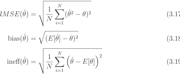
overall optimal estimate is the mean of all 100 best estimates. The dispersion of estimation
results is measured in Root-Mean-Square Deviation (RMSE). All results are reported in
Table 2.1.
The estimation results presented in Table 2.1 are very accurate as each estimate is close
to the associated true value. In fact, the estimation results of the SVVG model and SVLS
model are slightly weaker than that of the HJ model. It might be due to the fact that
estimating time-changed L´evy processes involves sampling with uncommon distributions.
Hence, the convergence is not as good as that which only involves sampling from the
Table 2.1: Estimation results on simulation data for three models
This table presents the estimation results of HJ, HVG, SVVG, SVLS model based on simulation data. For each model,
100 samples of daily data are simulated with the horizon of 20 years. For each sample, the estimates of parameters
are generated with the MCMC method. The best estimate is the mean value of all estimates. For each panel, the true
parameters predetermined are reported in the first row. The mean values of estimates of parameters are reported in
the second row. The dispersion of estimates is measured by RMSE and reported in the third row.
Panel A: HJ model
µ κ η σv ρ µy σy λy
True 0.05 1.50 0.36 0.25 -0.60 -3.00 2.50 0.02
Estimate 0.0510 1.5231 0.3589 0.2520 -0.5982 -3.0334 2.2353 0.0221
RMSE 0.0112 0.026 0.0231 0.0018 0.0101 0.0432 0.0582 0.0034
Panel B: HVG model
µ κ η σv ρ θ σ ν
True 0.05 1.50 0.36 0.25 -0.60 -0.05 0.25 2.5
Estimate 0.0504 1.5331 0.3643 0.2487 -0.5896 -0.0489 0.2513 2.5021
RMSE 0.0089 0.0342 0.0533 0.0135 0.0343 0.0065 0.0034 0.0532
Panel C: SVVG model
µ κ η σv θ σ ν
True 0.05 1.50 0.36 0.25 -0.05 0.25 2.5
Estimate 0.0491 1.5213 0.3598 0.2481 -0.503 0.2479 2.4891
RMSE 0.0079 0.0283 0.0481 0.0123 0.0068 0.0362 0.0682
Panel D: SVLS model
µ κ η σv α σ
True 0.05 1.50 0.36 0.25 1.85 0.25
Estimate 0.0493 1.5236 0.3581 0.2513 1.8483 0.2498
It is believed that the MCMC estimation method developed in this chapter is reliable
and accurate for the purpose of estimating time-change L´evy processes. We use two
representative time-changed L´evy models: the SVVG model and the SVLS model. The
results are accurate since the MCMC method can generate accurate samples of all latent
variables. The multi-dimensional problem does not seem to be a burden. We demonstrate
how to obtain accurate estimates of time-changed L´evy models with the MCMC method.
Hence, it becomes feasible to investigate whether time-changed L´evy models can provide
a better performance in terms of modelling asset returns.
2.4
Empirical results of time-changed L´
evy processes
This section will provide a series of empirical results, to show the advantages of using
time-changed L´evy processes in modelling returns. We carefully select the data set used
in this estimation experiment. MSCI indices are managed by Morgan Stanley, and are
often used as common benchmark portfolios for assessing funds’ performance. We choose
the World Index which captures large and mid cap representations across 23 developed
Markets and has been maintained since 1969.
Table 2.4 reports the summary statistics of daily log returns of the MSCI World index.
The sample data is collected from 2nd May 2001 to 31st December 2012. There are
3043 observations of returns reported in percentages in Table 2.4. The sampling period
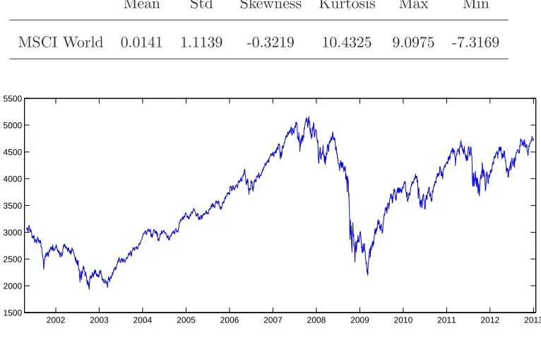
time series plot of the MSCI World Index. We can observe the bearish period after the
dot com bubble and the credit crunch period since 2008. There are also two booming
periods such as the recovering time after the crunch. The time series plot of log returns
presented in Figure 2.2 reveals the fact that the sampled returns are very volatile and
exhibit volatility clustering. The largest daily return is 9.10% on 13th October 2008 and
the biggest negative daily return is 7.32% on 15th October 2008.
Table 2.2: A summary of statistics of daily log returns of the MSCI World Index
This table reports the summary statistics of log returns of the MSCI World Index from 2nd
May 2001 to 31st December 2012. The continuously compounded returns are calculated as
the log difference successive index levels.
Mean Std Skewness Kurtosis Max Min
MSCI World 0.0141 1.1139 -0.3219 10.4325 9.0975 -7.3169
2002 2003 2004 2005 2006 2007 2008 2009 2010 2011 2012 2013
[image:43.595.116.499.400.639.2]1500 2000 2500 3000 3500 4000 4500 5000 5500
Figure 2.1: Time series plot of the MSCI World Index from 02/05/2001 to 31/12/2012
2001 2002 2003 2004 2005 2006 2007 2008 2009 2010 2011 2012 2013 −0.08
[image:44.595.116.520.110.316.2]−0.06 −0.04 −0.02 0 0.02 0.04 0.06 0.08 0.1
Figure 2.2: Time series plot of log returns of the MSCI World Index from 02/05/2001
to 31/12/2012
models, SVVG and SVLS, with the MCMC method presented in Section 2.2. The sample
data is the log returns of daily MSCI World index. As described before, the best estimate is
the expectation of the posterior distribution of the underlying parameter. We will sample
from the posterior distribution and use the empirical mean as a good approximation to
the expected value. For each estimation procedure, the sample size is 20,000. There is a
‘burn-in’ problem for the MCMC estimation method. This is because the MCMC method
relies on the fact that the stationary distribution can be obtained by using the transition
distribution. Hence, we need to ‘wait’ for some time before reaching the stable state. We
use 20,000 as the ‘burn-in’ sample size, which means we will generate 40,000 samples and
only use the last 20,000 samples to take the mean and standard deviation as the point
We report the estimated parameters in Table 2.3. Model used in the estimation
in-clude the Heston-Jump (HJ) model, the Heston-VG Jump-diffusion (HVG) model, the
time-changed Variance Gamma (SVVG) model, and the time-changed Log Stable (SVLS)
model. Estimates of parameters are reported with the associated standard errors which
are presented in parentheses. The expected mean estimated has a similar level as the
empirical mean which is 0.0141 reported in Table 2.4. It should not be the same as the
innovation distribution does not guarantee the Martingale property. The volatility level
also exhibits a similar level. It is interesting to check the jump intensity, based on the
estimation results. The jump intensity of the HJ model is about 0.0056∗252 = 1.4112
per year. Apparently, the jump intensity is far away from reality. This indicates the
necessity of using infinite activity L´evy processes. The average level of jump parts tends
to be negative as we observe µy =−2.3140. It is suggested that negative jumps are more
frequent and important. Hence, it also suggests that we should use the LS process as
this type of L´evy process only admits negative jumps with positive drift. The standard
errors obtained are very small except for those parameters of the jump structure of the HJ
model. This problem has also been reported in Eraker et al. (2002) and Li et al. (2008).
The estimates of L´evy models are more accurate, which demonstrates that the MCMC
method has a very good performance on estimating infinite activity L´evy processes.
To assess the performance of the estimation, we collect residuals from the last 100
itera-tions of each round of the MCMC estimation. The residuals should follow the standard
Table 2.3: Estimation results of the MSCI World Index
This table reports the estimation results given by the MCMC estimates method. The sample data is the MSCI World
Index collected from 02/05/2001 to 31/12/2012. Model used in the estimation include the Heston-Jump (HJ) model,
the Heston-VG Jump-diffusion (HVG) model, the time-changed Variance Gamma (SVVG) model, and the time-changed
Log Stable (SVLS) model. Estimates of parameters are reported with the associated standard errors which are presented
in parentheses.
HJ HVG SVVG SVLS
µ 0.0135 µ 0.0217 µ 0.0327 µ 0.0311
(0.0010) (0.0009) (0.0012) (0.0013)
κ 0.3541 κ 0.3125 κ 0.6421 κ 0.5982
(0.0055) (0.0036) (0.0052) (0.0063)
η 0.8461 η 0.8762 η 0.9874 η 0.9012
(0.0832) (0.0810) (0.1032) (0.0961)
σv 0.1235 σv 0.1323 σv 0.1459 σv 0.1682
(0.0013) (0.0016) (0.0021) (0.0091)
ρ -0.3132 ρ -0.3562 σ 0.5434 α 1.7654
(0.0201) (0.0108) (0.0042) (0.0014)
µy -2.3140 σ 0.4325 θ -0.1754 σ 0.7658
(0.8931) (0.0138) (0.0132) (0.0047)
σy 3.1596 θ -0.1340 ν 4.9812
(1.1310) (0.0063) (0.1302)
λy 0.0056 ν 5.3225
estimation can be evaluated by testing how close the residuals are away fromN(0,1). In
Figure 2.3, the Kernel Density estimator of the HJ model is presented with the
corre-sponding QQ plot. Obviously, the HJ residuals are not normally distributed. The main
differences appear to be the high moments and tail behaviour. According to the QQ plot
in Figure 2.3, the left tail is extremely away from the Normal predication, which suggests
that the HJ model has a poor performance on fitting the negative jumps exhibited from
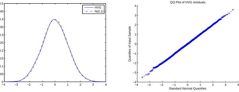
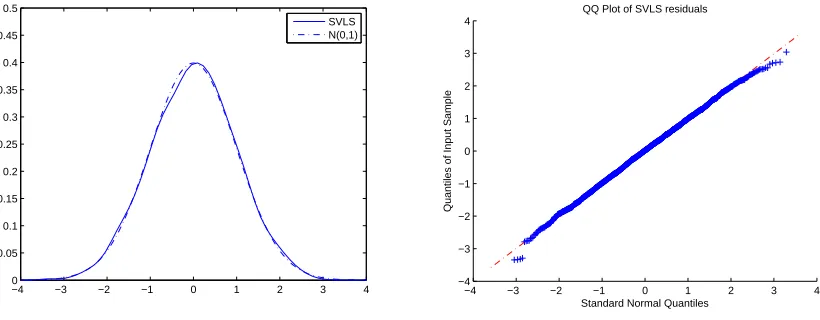
the market. Figure 2.4, 2.5 and 2.6 present the Density estimators and QQ plots for HVG,
SVVG and SVLS models, respectively. Actually, the HVG model provides the best fit;
the other two time-changed L´evy models also show good fit, but the tail behaviours are
slightly different from Normal distribution. As discussed before, the time-changed L´evy
models do not admit the leverage-effect. Hence, the tail behaviour might be slightly
dif-ferent. The correlation between the spot price and the volatility is about −0.3562, which
is not very strong. Our estimation results of time-changed L´evy models might become
worse if a different data set with high leverage-effect is used.
−4 −3 −2 −1 0 1 2 3 4 0 0.05 0.1 0.15 0.2 0.25 0.3 0.35 0.4 0.45 0.5 HJ N(0,1)
−4 −3 −2 −1 0 1 2 3 4 −4 −3 −2 −1 0 1 2 3 4
Standard Normal Quantiles
Quantiles of Input Sample
[image:47.595.98.504.509.669.2]QQ Plot of HJ residuals
−4 −3 −2 −1 0 1 2 3 4 0 0.05 0.1 0.15 0.2 0.25 0.3 0.35 0.4 0.45 0.5 HVG N(0,1)
−4 −3 −2 −1 0 1 2 3 4 −4 −3 −2 −1 0 1 2 3 4
Standard Normal Quantiles
Quantiles of Input Sample
[image:48.595.97.504.154.311.2]QQ Plot of HVG residuals
Figure 2.4: Kernel density and QQ plot of the residuals of the HVG model
−4 −3 −2 −1 0 1 2 3 4 0 0.05 0.1 0.15 0.2 0.25 0.3 0.35 0.4 0.45 0.5 SVVG N(0,1)
−4 −3 −2 −1 0 1 2 3 4 −4 −3 −2 −1 0 1 2 3 4
Standard Normal Quantiles
Quantiles of Input Sample
QQ Plot of SVVG residuals
[image:48.595.95.504.471.632.2]−4 −3 −2 −1 0 1 2 3 4 0 0.05 0.1 0.15 0.2 0.25 0.3 0.35 0.4 0.45 0.5 SVLS N(0,1)
−4 −3 −2 −1 0 1 2 3 4 −4 −3 −2 −1 0 1 2 3 4
Standard Normal Quantiles
Quantiles of Input Sample
[image:49.595.94.504.106.266.2]QQ Plot of SVLS residuals
Figure 2.6: Kernel density and QQ plot of the residuals of the SVLS model
Apart from the graphical evaluation, a statistical test is also needed. A simple choice is
the One-sample Kolmogorov-Smirnov test. We apply the Kolmogorov-Smirnov test to the
final 100 iterations to check whether residuals follow the standard Normal distribution.
In Figure 2.4, percentage of rejections is reported in the second column and the associated
mean value of p-value is reported in the third column. For the HJ model, the KS test
reject 96% of sets of residuals. The average p-value is only 0.0086. This result is similar to
that in Li et al. (2008). Apparently, the HJ model cannot capture the behaviour of index
returns. This is consistent to the results observed in Figure 2.3. The winner, as shown
in Table 2.4, is the HVG model which has only 11 sets of residuals rejected in the KS
test. The residuals produced by the HVG model is very close to standard Normal. The
two time-changed L´evy models also provide good fit. For instance, 31 sets of residuals
produced by the SVVG model are rejected while only 23 sets are rejected for the SVLS
model. The corresponding mean p-values are 0.2781 and 0.3539, respectively. The above
in capturing return dynamics. Pure time-changed L´evy models are slightly weaker than
the stochastic volatility models with infinite L´evy jumps. This might be due to the
absence of the Leverage-effect. If time-changed L´evy models subordinated by pure L´evy
jumps are used, it is possible to achieve better performance. It is also suggested that the
[image:50.595.182.419.402.519.2]LS process can provide good performance in modelling index returns.
Table 2.4: Empirical results of Kolmogorov-Smirnov Test
We test four models including HJ, HSV, SVVG, and SVLS, based on the daily data of the MSCI
World index. For each of the final 100 iterations, the model residuals are collected based on the
estimated model parameters. We apply the Kolmogorov-Smirnov test to the final 100 iterations to
check whether residuals follow the standard Normal distribution. Percentage of rejections is reported
in the second column and the associated mean value of p-value is reported in the third column.
percentage of rejection(%) mean p-value
HJ 96 0.0086
HVG 11 0.4675
SVVG 31 0.2781
SVLS 23 0.3539
Due to the advantage that MCMC estimation can simulate latent variables, we can also
have a look at the estimated latent variables such as volatility to check the accuracy of
fit. In Figure 2.7, the estimated volatility plots are depicted for the four models used in
our experiment. According to the return time series plot of the index shown in Figure 2.2,
the most volatile period is between 2008 and 2009 when the credit crunch happened. Our
variation of volatilities. We can observe extreme large jumps between 2008 and 2009 as
well as in late 2011.
2002 2004 2006 2008 2010 2012 0
0.5 1 1.5
HJ: Estimated Volatilities
2002 2004 2006 2008 2010 2012 0 0.2 0.4 0.6 0.8 1
HVG: Estimated Volatilities
2002 2004 2006 2008 2010 2012 0 0.2 0.4 0.6 0.8 1 1.2 1.4 1.6
SVVG: Estimated Volatilities
2002 2004 2006 2008 2010 2012 0 0.2 0.4 0.6 0.8 1 1.2 1.4 1.6
[image:51.595.94.504.155.484.2]SVLS: Estimated Volatilities
Figure 2.7: Estimated volatilities of HJ, HVG, SVVG, and SVLS models
This empirical experiment shows the benefit of adopting infinite activity L´evy processes in
modelling index returns. The HVG, SVVG and SVLS model all show very good accuracy
of fit. Although time-changed L´evy models do not outperform the stochastic volatility
model with infinite activity L´evy jumps (HVG), this might be due to the absence of
the Leverage-effect. For the index return data we choose, the correlation between the
the HVG model and other two time-changed L´evy models is not very significant. It
seems that the only reason we should keep diffusion is because we want to generate the
Leverage-effect. If proper time-changed L´evy models that admit the Leverage-effect can
be developed, the diffusion component can be dropped without losing good fit.
2.5
Conclusion
Continuous-time models have been widely used in capturing the return dynamics of
indi-vidual stocks and indices. The jump-diffusion model plays an important role for portfolio
allocation problem as it can model both small and large movements of return series.
However, the jump-diffusion models cannot achieve accurate fit of market returns.
Time-changed L´evy processes provide a much broader and more flexible class of models for
capturing asset price dynamics. This chapter investigates the empirical advantages of
using L´evy processes for modeling index returns. The MCMC techniques developed in
this chapter is a further extension of the MCMC method for stochastic volatility models
in Li et al. (2008). The advantage of infinite activity L´evy processes is allowing an infinite
number of jumps within any finite time interval. Hence, all jumps or movements of returns
with different sizes can be captured by time-changed L´evy processes, especially for highly
frequent discontinuous movements in stock prices. The MCMC estimation method can
approximate model parameters, latent variables and jump variables of time-changed L´evy
processes. Based on empirical analysis, we show that time-changed L´evy models can
diffusion component can be omitted as infinite activity L´evy processes can capture all
Chapter 3
An Empirical Study of Multivariate
MCMC Estimation on L´
evy
processes
In Chapter 2, we have provide a detailed investigation on estimating the one-dimensional
time-changed L´evy processes with the Markov Chain Monte Carlo ( MCMC ) technique;
However there is still a gap in this field. There is no efficient method that has been applied
for multi-dimensional processes. The extreme complexity of high-dimensional estimation
is the huge obstacle. Wether or not L´evy processes should be used for portfolio problem
can only be answered with the development of estimation technique.
im-plemented. The interest in multidimensional asset models based on L´evy processes is
motivated by the importance of capturing market shocks using more refined distribution
assumptions compared to the standard Gaussian framework, incorporating skewness and
kurtosis. From a risk management perspective, in fact, the focus is specifically on the
tails of the stock return distribution, and commonly used risk measure such as Value
at Risk and intra-horizon Value at Risk aim at quantifying the economic impact of rare
events. Further, for regulatory purposes these risk measures are usually obtained for short
time horizons (i.e. 10 days), over which the effects of stochastic volatility are in general
negligible (mainly due to the diffusive nature of the processes used for the modelling of
volatility trends). In this respect, L´evy processes can offer a natural and robust approach
to model distribution tails compared to the Brownian motion, especially over the short
period, as they allow for extreme outcomes to happen more frequently. However,
con-sistent and efficient estimation procedures, which are essential part of the calculation of
relevant risk measures, can be problematic for L´evy processes as extensively documented
in Cont and Tankov (2004). For example, these issues are exacerbated by increasing the
dimension of the parameter space, which would be necessary in order to accommodate
for the multivariate modelling required at portfolio level.
Linear transformations have been used extensively in the literature to build multivariate
L´evy processes as these processes are invariant under such a transformation, and therefore
their characteristic function and characteristic triplet can be obtained in a straightforward
model each risk driver as a linear combination of two independent processes representing
respectively the systematic factor and the idiosyncratic shock, so that dependence
be-tween assets in a given portfolio is originated by the common component of the overall
risk. Contributions based on linear transformations started with Vasicek (1987) for the
case of Brownian motions; for the extension to L´evy processes we mention, Ballotta and
Bonfiglioli (2014) and Luciano and Semeraro (2010). In more details, Luciano and
Se-meraro (2010) apply the factor approach to the asset log-returns process, which allows to
choose any L´evy process as factor processes, and encompasses any class of L´evy processes,
from subordinated Brownian motions to jump-diffusion processes. Linear transformations
have also been used in the literature to build multivariate subordinators and therefore
alternative multivariate versions of subordinated Brownian motions; this is the case of
Luciano and Semeraro (2010) who offer a general construction for subordinated Brownian
motions, such as the Normal Inverse Gaussian (NIG) and the Carr-Geman-Madan-Yor
(CGMY) processes. Extensions to a factor-based subordinated Brownian motion are
pro-posed by Luciano (2013) in order to incorporate additional dependence properties.
A common trait to all these contributions is the presence of (either explicit or implicit)
convolution conditions, which allow to separate the dependence structure from the
distri-bution of the margin processes. However, as argued by several authors such as Eberlein
et al. (2008), this feature, although intuitive, leads to a biased view of the dependence in
place as it reduces the flexibility of the factor model, and fails to recognize the different
model of Ballotta and Bonfiglioli (2014) these convolution conditions are not necessary
for the model to retain its mathematical tractability, its relative flexibility in
accommo-dating a wide range of dependence structures, positive and negative linear correlation and
a parsimonious number of parameters.
As we try to fill the gap, we propose an efficient estimation procedure for the
multi-variate (exponential) L´evy processes model of Ballotta and Bonfiglioli (2014) with risk
management applications type in view, specifically the computation of Value at Risk and
intra-horizon Value at Risk for portfolios of dependent assets. Thus, we focus on the
model estimation under the physical probability measure, which is in fact non-trivial as
the common and the idiosyncratic factors driving the margins are not directly observable
in the market. In order to simplify this problem, although other approaches are possible,
here we follow standard market practice and assume that the common factor representing
systematic risk can be well-proxied by the returns on a broad-based index.
The first main contribution of this chapter is the robust MCMC estimation procedure
for the multivariate L´evy processes model. Simulation study shows that this approach
can provide very accurate joint identification of L´evy jumps and stochastic volatility.
we demonstrate the accuracy and stability of the MCMC method based on simulation
data. This enables us to explore whether time-changed L´evy model can generate better
fit, compared with existing stochastic Jump-diffusion models. To assess this estimation
procedure, we also implement a standard one-step maximum likelihood approach in which