Using machine learning algorithms to improve traffic state estimation : a study on the usability of machine learning techniques in traffic state and speed estimation

Full text

(1)Using machine learning algorithms to improve traffic state estimation A study on the usability of machine learning techniques in traffic state and speed estimation. Master thesis. Antoon Dommerholt August 29, 2019.

(2) Colophon Title: Subtitle:. Using machine learning algorithms to improve traffic state estimation A study on the usability of machine learning techniques in traffic state and speed estimation.. Date:. August 29, 2019. Author: Student number: Email: Telephone:. A.J. (Antoon) Dommerholt s1026534 [email protected] 06 465 88 456. Institution: Faculty: Research group: Master: Track:. University of Twente Engineering Technology (CTW) Centre for Transport Studies (VVR) Civil Engineering and Management Transport Engineering and Management. UT–supervisor: Supervisor:. Prof. Dr. Ir. E.C. (Eric) van Berkum Dr. Ir. L.J.J. (Luc) Wismans. 2.

(3) Summary Traffic state is defined by the traffic variables intensity, speed and density. When two of the three defining variables are known a traffic state can be determined. When only one of the variables is known, additional information is needed for traffic state estimation. INWEVA is an overview of intensities on the Dutch national roads. For the parts of the road network that are not covered by detection loops, intensities are estimated by a model. Since only an estimation of intensities is known for these road sections, traffic state cannot be determined directly. Additional procedures have to be taken to estimate speed, and thus defining traffic state. In this research the relation between intensities and speeds is studied. This research aims to give a good estimation of speed, based on intensity data only. When speeds are known, it can be determined whether or not congestion occurs, and traffic state is defined. The estimations of traffic state are made by inputting intensities into machine learning models. The main question for this research is given below and is answered by researching the appropriate machine learning technique for traffic estimation and researching if there are additional attributes that may improve estimation. The last subquestion tries to find an answer to whether or not characteristics of road section are transferable to other road sections, in order to train models on other road sections than they will be tested on. How can machine learning techniques estimate traffic state based on intensity data? Literature review The relation between intensity and speed is given by the fundamental diagram (figure 2.1). This fundamental diagram consists of two parts, a free flow branch and a congested branch. In both these branches the same intensities occur, the speed, however, is different. Because the same value for intensity can belong to different speeds, speed cannot be directly derived from intensities. Different researches have tried to make estimations of traffic state, only having one defining variable available. This can be the case in speed estimation, only knowing intensities (in cases of single detection loop data), or in estimating intensities, only having speed data available (e.g. from floating car data). All methods that are doing these estimations need to have additional input. It is rather impossible to find a direct relation between the traffic state variables, based on only knowing one of them. Many different techniques for machine learning are available. Two main categories in supervised machine learning are decision tree learning models (DTL) and artificial neural networks (ANN). Regression is a mathematical approach that also tries to find relation between the input and output variables. Machine learning models are trained on exemplary data and tested on another set for their performance. Recurrent machine learning models perform well at capturing patterns where time sequences are involved. Methodology Data from NDW (Nationale Databank Wegverkeersgegevens) is used for training the machine learning models. This NDW data, that consists of intensities and speeds, is used as input to the model. This one minute aggregate data is aggregated to a 15-minute resolution and prepared to be used by the machine learning software. A set of locations is selected for this research and this is researched over a timespan that covers many situations. The estimation of traffic states consists of two parts: congestion estimation and speed estimation. The performance of congestion estimation is measured by the f-score, which combines precision and recall. For speed estimation the performance measure is the root mean squared error (RMSE), which gives an indication of how much the estimation is on average apart from the measured value.. 3.

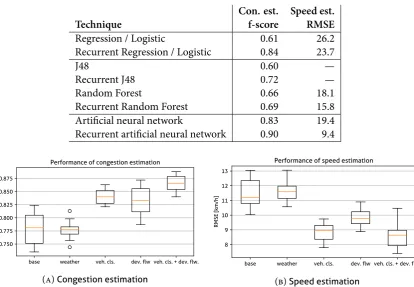
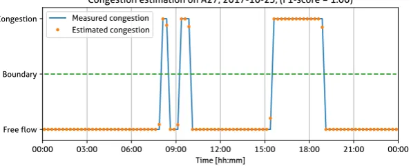
(4) 4 Different types of machine learning models are tested, using the weka software, for their performance. Before testing machine learning models, regression models are tested. The inputs that are used in the model are only intensities. Intensities from the selected location and an upstream and downstream location. For these three locations the input is given for the time that it is estimated, as well as the intensities on the interval before it and after it. The different models are compared to each other using the performance measures. Additional input attributes are tested for their influence to the model outcomes. The additional factors tested are influence of the weather, deviation in the intensity data and the percentage of long vehicles. The outcomes of the attribute testing is compared to the values for testing only on intensities. The last part of this research consists of testing models that are trained on data from multiple road sections. In the first place a model is tested that was trained on a combined training set of all roads, including the training set of the road that is tested on. In the second place a model is tested that is trained on a dataset that does not contain instances of the road section that is tested. These results are compared to earlier results. In order to combine data sets, road specific characteristics were added, such as speed limit, distance to up– and downstream location, number of lanes and what kind of bottleneck is present. Also, the intensities are scaled to a percentage of the roads capacity, in order to make the intensities of the different roads comparable. Data The data that is used, is NDW data that comes from MONICA or MONIBAS detection loops. MONIBAS is data that is already further processed than MONICA data. MONICA, however, more often contains data on vehicle length, this is one of the reasons also often MONICA data is used. Whenever MONICA data is used, it is processed in the same way MONIBAS data is processed, so both sources can be used together. Not all data does contain information on vehicle classes, most of the locations that are selected do have information on this. The NDW data comes in a resolution of one minute. The input for the model in this case is 15 minutes, so it has to be aggregated to this resolution. Also the different lanes on the road are aggregated. For the data that is used for congestion estimation, an instance is considered congested when the speed is below 70 km/h. From this data instances are formed that can be used as an input to weka. A total of twelve locations are selected for this research. These locations have a variety for several road situations. Most of the selected locations contain a bottleneck. Six have a decrease in the number of lanes, four have an on-ramp and two locations do not have a bottleneck at the site. A total of nine weeks of data is used divided throughout the year. Three weeks are taken from October 2017, three weeks from January 2018, and three weeks from April 2018. Results Different kind of models are tested and scored using the performance measure. Testing has been done both in congestion estimation as in speed estimation. Testing these models took place at a road section on the A27. A summary of the results of this model testing is shown in table 1. In all cases the recurrent version of the model performs better than the non-recurrent version. Recurrent neural networks (RNN) show both in congestion as in speed estimation the best results. A f-score of 0.90 is found for congestion estimation and a RMSE of 9.4 (km/h) for speed estimation. Because RNNs score highest, they are used for all other testing in this research. Weather, vehicle classes and deviation within the intensity data have been tested as additional input attributes for their influence on the performance of the model. The road that is tested on is a section on the A58. This road section was chosen because this road section has information about vehicle classes available. In figure 1 the results of this testing is shown. Information about weather does not lead to improvement of the model. Adding information on vehicle classes and deviation in the intensity data does improve the results significantly. Combine the latter two even gives slightly better results..

(5) 5 Table 1: Results of model testing on the A27. Technique Regression / Logistic Recurrent Regression / Logistic J48 Recurrent J48 Random Forest Recurrent Random Forest Artificial neural network Recurrent artificial neural network. Speed est. RMSE 26.2 23.7 — — 18.1 15.8 19.4 9.4. Performance of speed estimation. Performance of congestion estimation. 13. 0.875. 12 RMSE [km/h]. 0.850 F1 score. Con. est. f-score 0.61 0.84 0.60 0.72 0.66 0.69 0.83 0.90. 0.825 0.800 0.775 0.750. 11 10 9 8. base. weather. veh. cls.. dev. flw veh. cls. + dev. flw.. (a) Congestion estimation. base. weather. veh. cls.. dev. flw veh. cls. + dev. flw.. (b) Speed estimation. Figure 1: Results of adding additional input attributes in congestion and speed estimation on the A58. Testing on a model that is trained on a training set that is combined from multiple road sections lead to scores that are comparable to the scores of models that are trained on a single road section. On average the results were slightly worse, but on average these changes are not significant. When a model that is trained on data, in which the road section on which is tested, is not included, results become very bad. There is hardly any estimation power left and these models should not be used for traffic state estimations. An overview of all results on all road is given in table 2. Conclusions For traffic state estimation based on intensity data, the RNN is the most suitable machine learning technique. Because of the fact that traffic state is a temporal sequence, recurrent models are always preferred. The RNN is capable of estimating traffic state, based on intensity data. Best results are found in cases of clear bottlenecks, where all intensity data is available, for example at lane drops. Weather input was found not to improve the results of the model significantly. Adding information on vehicle length and deviation in intensity data did result in a significant improvement in performance. A combination of the latter two resulted in even slightly better results. In congestion estimation the f-score improved by 7.8%, and in speed estimation the RMSE improved even 22.9%. Having a model trained on a larger training set than the road section only, will lead to comparable results as when it is trained on a specific road section only. But when the training set does not contain instances from the road section that it is tested on, the model performs badly. This shows that the RNN is not capable of transferring the characteristics from one road section to the other. Neural networks seem not to be able to interpolate and extrapolate well. Discussion In the context of estimating speeds using intensity data of INWEVA, the results of this research cannot be used. In order to do so, a model should be trained on known data (from other road sections) as the use case. This research showed that doing that does not result in good estimations. For cases where it is.

(6) 6 Table 2: Results of different models on all road sections. (The underlined values indicate the road and value this model was trained on.). Road A01_03 A02_02 A04_01 A04_02 A07_01 A27_02 A27_03 A28_01 A28_02 A58_01 A58_02 A58_03. Congestion Estimation (f-score) RNN RNN RNN RNN base1 add. attr.2 merged3 other4 0.72 0.69 0.68 0.07 0.66 0.66 0.72 0.50 0.77 0.78 0.76 0.24 0.86 0.92 0.93 0.42 0.62 0.64 0.56 0.16 0.90 0.89 0.85 0.66 0.39 0.52 0.48 0.18 0.48 0.50 0.51 0.20 0.58 0.23 0.26 0.04 0.81 0.84 0.87 0.26 0.78 0.87 0.74 0.51 0.87 0.89 0.86 0.53. Speed Estimation (RMSE) RNN RNN RNN RNN base add. attr. merged other 11.2 11.3 12.3 82.4 9.7 9.2 10.1 13.8 10.5 11.8 11.2 29.6 8.8 6.8 7.5 51.5 9.4 9.2 11.2 19.0 9.4 10.5 11.3 39.6 13.5 13.1 13.3 54.3 15.1 14.4 14.8 22.0 6.8 6.2 8.1 31.1 10.4 9.7 11.3 44.7 11.5 8.2 12.2 16.5 10.0 9.2 9.8 14.6. possible to have a base measurement of intensities and speeds, this research shows, however, that for situations on that same road section where only intensities are known, it is possible to make proper estimations of the speed. The methodology and the data have caused some limitations to the scope of this research. A lack of data caused that situations with ramps had incomplete intensity data, because many ramps were not measured. A limitation from the methodology is the limited number of locations that were chosen. By choosing more road sections, the dataset could have been a better representation of the Dutch motorway network. A limitation for the practical use is that data from the future time steps are used for estimation, this makes it impossible to apply the model real time. There are a few directions for future research that can be followed from this research. The most interesting direction is carrying out the same research, but the other way round. Then a model would be made to estimate intensities, based on speeds, using machine learning techniques. Comparing those results to this research could give more insight in the relation between intensity and speed.. 1. Trained on intensity data only. Having added additional attributes. 3 Instances from all roads are included in both the training set as the test set. 4 Tested on a model that is trained on a model that does not contain instances from the same road as it is tested on. 2.

(7) Contents Summary. 3. 1. Introduction 1.1 Context . . . . . . . . . . . . . . . . . . . . . . . . . . . . . . . . . . . . . . . . . . . 1.2 Research objective and research questions . . . . . . . . . . . . . . . . . . . . . . . . 1.3 Thesis outline . . . . . . . . . . . . . . . . . . . . . . . . . . . . . . . . . . . . . . . .. 8 8 9 9. 2. Theoretical framework 10 2.1 Traffic states . . . . . . . . . . . . . . . . . . . . . . . . . . . . . . . . . . . . . . . . 10 2.2 Machine learning in traffic engineering . . . . . . . . . . . . . . . . . . . . . . . . . . 13. 3. Methodology 3.1 Data collection . . . . . . . . . . 3.2 Testing several models . . . . . . 3.3 Testing additional attributes . . . 3.4 Testing on a set of multiple roads. 4. 5. . . . .. Data collection 4.1 Data Sources . . . . . . . . . . . . 4.2 Locations . . . . . . . . . . . . . . 4.3 Time periods . . . . . . . . . . . . 4.4 Obtaining and processing the data 4.5 Information on the road sections .. . . . .. . . . .. . . . .. . . . .. . . . .. . . . .. . . . .. . . . .. . . . .. . . . .. . . . .. . . . .. . . . .. . . . .. . . . .. . . . .. . . . .. . . . .. . . . .. . . . .. . . . .. . . . .. . . . .. . . . .. . . . .. . . . .. . . . .. . . . .. 19 19 21 22 22. . . . . .. . . . . .. . . . . .. . . . . .. . . . . .. . . . . .. . . . . .. . . . . .. . . . . .. . . . . .. . . . . .. . . . . .. . . . . .. . . . . .. . . . . .. . . . . .. . . . . .. . . . . .. . . . . .. . . . . .. . . . . .. . . . . .. . . . . .. . . . . .. . . . . .. . . . . .. 23 23 25 25 26 27. Testing several machine learning techniques 5.1 Tested road section . . . . . . . . . . . . 5.2 Congestion estimation . . . . . . . . . . 5.3 Speed estimation . . . . . . . . . . . . . 5.4 Validation on other roads . . . . . . . .. . . . .. . . . .. . . . .. . . . .. . . . .. . . . .. . . . .. . . . .. . . . .. . . . .. . . . .. . . . .. . . . .. . . . .. . . . .. . . . .. . . . .. . . . .. . . . .. . . . .. . . . .. . . . .. . . . .. . . . .. . . . .. 29 29 30 36 39. . . . . .. . . . . .. 6. Additional input attributes 41 6.1 Tested road section . . . . . . . . . . . . . . . . . . . . . . . . . . . . . . . . . . . . . 41 6.2 Tested additional data . . . . . . . . . . . . . . . . . . . . . . . . . . . . . . . . . . . 43 6.3 Validation on other road sections . . . . . . . . . . . . . . . . . . . . . . . . . . . . . 45. 7. Multiple road input 47 7.1 Attribute selection . . . . . . . . . . . . . . . . . . . . . . . . . . . . . . . . . . . . . 47 7.2 All roads in both sets . . . . . . . . . . . . . . . . . . . . . . . . . . . . . . . . . . . . 47 7.3 Different roads in train set and test set . . . . . . . . . . . . . . . . . . . . . . . . . . 48. 8. Conclusions and discussion 50 8.1 Conclusions . . . . . . . . . . . . . . . . . . . . . . . . . . . . . . . . . . . . . . . . 50 8.2 Discussion . . . . . . . . . . . . . . . . . . . . . . . . . . . . . . . . . . . . . . . . . 52. References. 55. 7.

(8) 1 Introduction In this introduction the context of the research is explained, the objective and the research questions are defined.. 1.1 Context Two elements that define a traffic state are the intensity on a road and the speed that is driven. Those two factors do not have a one-to-one relationship, which means that when only one of the two is known, the other cannot be derived from it. In figure 1.1a the progress of both intensity and speed during a typical day are shown. What can be seen here is that a specific value for intensity does not always correspond to the same speed. This can be seen more clearly in the fundamental diagram in figure 1.1b, where speed / intensity combinations are plotted. Because the same intensity can belong to a low speed (around the red line) or to a higher speed (around the green line), having knowledge about a specific value for intensity will give no certainty on the corresponding speed. 140. V (km/h). 120 100 80 60 40 20 0. 0. 500. 1000. 1500. 2000. 2500. Q (veh/h/lane) (b) The fundamental diagram. (a) Progress of intensity and speed. Figure 1.1: Example of the progress of intensity and speed (DatMobility, 2017) and a fundamental diagram (Treiber & Kesting, 2013), showing that the same intensity does not always correspond to the same speed.. In the Netherlands there is an overview of intensities on the Dutch national roads, which is called INWEVA (meaning: intensities on road stretches). For a significant part the intensities are measured by detection loops, but there also is a part of the network that is not covered by loops. For these uncovered road stretches the intensities are estimated by a model (Rijkswaterstaat, 2018). For the measured road stretches both intensities and speeds are known, since the loops that are used in the Netherlands are double loops, that can both measure intensity and speed. For the unmeasured road stretches all that is available is a modelled estimation of intensity. As mentioned before, with only intensity data, speed cannot be determined evidently. This makes it also difficult to determine whether or not congestion takes place at a road stretch, with intensity data only. Being able to estimate or predict congestion state and speed could hugely improve the INWEVA data for the Dutch national roads. When speed were to be linked to the corresponding intensity data, a complete picture of traffic state for the national road system could be given. Also only being able to link congestion to the intensities would be of great benefit, since it can be identified where bottlenecks are located and when they are likely to be congested. A research on identifying congestion based on intensity data was conducted by DatMobility (2017). The intensity data that was used was measured traffic intensity with 15 minute intervals. An artificial neural network was used to find out if it is possible to predict whether or not congestion is occurring, based on these modelled intensities. Some good results were found at locations where often congestions 8.

(9) Research objective and research questions. 9. occurred by clearly identifiable bottlenecks. There is, however, improvement possible on the method and the techniques used. This research builds on the research done by DatMobility (2017). It has the same goal, which is identifying traffic state, based on 15 minute intensity data. Also machine learning techniques are used in order to achieve this goal, but more advanced techniques were applied to the problem. Also this research goes one step further in estimation of traffic state, since it does not only try to detect congestion, but does also try to give an indication of the speed at locations. Further this research is not limited to single road sections, but aims to make a framework that can estimate traffic state throughout the whole network of motorways in the Netherlands.. 1.2 Research objective and research questions Before giving an overview on how the research is conducted the objective and research questions are formulated. The aim of this research is using machine learning techniques to give an estimation on traffic state, based on intensity data. This will be useful for cases were only intensity data is known and more information is desirable, such as the modelled intensities on the parts of the Dutch national roads were traffic monitoring is not present. The formal aim of this research is generalized from this context and is as follows: Using machine learning techniques to give an estimation of congestion state and speed, based on intensity data. This aim has been formulated as a research question that was attempted to answer in the research. To be able to answer this research question, it is divided into three subquestions, which together provide for an answer to the main question. The main question is defined as follows: How can machine learning techniques estimate traffic state based on intensity data? The main question is divided into subquestions as follows: 1. What is the appropriate machine learning technique for estimating traffic state? 2. What input variables are important in the machine learning process? 3. How can a general approach be made for estimating congestion state and speed based on 15 minute aggregate intensity data on Dutch highways?. 1.3 Thesis outline This thesis starts with a literature review, which is focused on how traffic state is usually estimated and what variables play a role in it. Also different types of machine learning algorithms are discussed. A few examples of how machine learning can be combined with traffic engineering from literature are discussed. In the methodology it is explained how this research is conducted. All steps that are taken are explained and motivated. The methodology is followed by a chapter on data collection. Choices for which data are used, is motivated. Also the process how the data is prepared is described. In chapters 5 to 7 the results of the research are presented. This starts with testing different types of machine learning models, in which regression models, decision tree learning models and artificial neural networks are tested for its suitability in traffic state estimation for a particular road section. The best tested model is used for additional attribute testing. In the last phase of this research it is tested if the model still has estimating power when the model is trained on multiple road sections and when the model is trained on road sections that are not included in the test set. In the conclusions the research questions are answered. In the discussion it is discussed how these findings can be of practical use in the outlined context. Also the limitations are discussed and recommendations for future work are given..

(10) 2 Theoretical framework 2.1 Traffic states Traffic state is defined by the variables speed, flow, and density. The relation between these will be discussed in this chapter, by using the fundamental diagram. This is followed by a short view on how traffic state can be estimated, when not all variables are known. 2.1.1 Fundamental diagram In highway traffic there are roughly two traffic regimes. In the free flow regime densities are low enough that congestion does not appear and single vehicles can to some extend choose their own speed. In this traffic regime speeds will generally be high. In the congested state speeds are lower than the free flow speed. The maximum intensity is found at the place where the congested regime and the free flow regime meet. This can be seen in figure 2.1 at the place where the green and the red line intercept. In traffic state estimation all traffic variables that define the current traffic state need to be estimated (Wang & Papageorgiou, 2005).. 140. V (km/h). 120 100 80 60 40 20 0. 0. 500. 1000. 1500. 2000. 2500. Q (veh/h/lane) Figure 2.1: The relation between intensity and speed (one minute intervals) in the fundamental diagram (Treiber & Kesting, 2013).. The fundamental diagram of traffic describes the relation between the three variables that define traffic state in stationary conditions. Those variables are speed (𝑣), density (𝜌) and intensity or flow (𝑞), that relate to each other 𝑞 = 𝜌𝑣. Theory of the fundamental diagram assumes that these three variables satisfy the equations 2.1 and 2.2 (Seo, Bayen, Kusakabe, & Asakura, 2017). 𝑣 = 𝑉(𝜌). (2.1). 𝑞 = 𝜌𝑉(𝜌) = 𝑄(𝜌). (2.2). In which 𝑉 and 𝑄 represent the fundamental relations between speed-density and flow-density respectively. This fundamental diagram plays an important role in traffic state estimation, because it is the core of traffic flow theory (Seo et al., 2017). Knowing this relation means that two of the three traffic state variables are needed to define a traffic state. The third variable can be deducted from the other two, assuming a stationary and homogeneous flow. A visualisation of one of those fundamental relations is shown in figure 2.1. Measurements of speedintensity combinations are shown as black dots. In this relation between traffic intensity and speed two 10.

(11) Traffic states. 11. different traffic states can be distinguished. The green line indicates the free flow condition, while the red line shows congested traffic flow. As can be seen in figure 2.1 a certain intensity does not always belong to the same speed. Roughly almost every intensity can belong to the free flow regime, or to the congested regime, with its corresponding speeds. This means that only measuring intensity will not automatically lead to knowing the speed or the current traffic state. Knowing the regime of the current traffic state would already give a much better view on the speed of traffic. Therefore separation of intensities in either the free flow or the congested regime would already be very beneficial. Another way to determine traffic state when only intensity is known, is finding the density. Finding density, however, is difficult with the current technology. In order to find the density the number of vehicles on a certain road stretch in one moment needs to be determined. This is only possible when each vehicle is located at the same moment. Approaches of this can only be made when many vehicles would continuously transmit their location, which is not the case at the moment. Therefore, to estimate traffic state flow and speed are generally used. What can be seen in figure 2.1 is that in the free flow traffic regime is that the green line is rather flat. This indicates that within in the free flow regime vehicles drive their maximum speed (speed limit), even when the intensity increases. Only with lower intensities in the free flow regime, the variation in speeds is higher, which is probably caused by freight traffic at night, which drive at lower speeds. The flow-speed dots in the fundamental diagram are aggregate values, so the speed is a average speed for a certain interval. This means that when the share of long vehicles (with a lower speed limit) in the interval is higher, the average speed will be lower, even though there are free flow conditions. An interesting place in figure 2.1 is the place where the red and green line meet. This is the place with the maximum capacity during congested situations. In free flow conditions the capacity can be higher. When the traffic state changes from free flow conditions to congested conditions a capacity drop occurs (Treiber & Kesting, 2013). This means that as long as there is a congested situation, the free flow capacity cannot be reached. If the dots between consecutive flow-speed combinations were connected the effects of hysterics could be shown and it could be seen that the intensity needs to drop significantly during congested situations, before the system can recover again to free flow conditions. Because of these sequences, it is important to look at the history of traffic state when defining a current traffic state. For the relation between intensity and speed, also the location and time play a role and the fundamental diagram function can be expressed as 𝑄(𝜌, 𝑡, 𝑛, 𝑥), in which 𝜌 is the density, 𝑡 the time, 𝑛 the type of vehicle and 𝑥 the location (Seo et al., 2017). Therefore factors as these are important to consider when discussing the intensity-speed relation. For the location it is important to know the road configuration, e.g. the number of lanes, whether it is located just before or after a bottleneck or if it is on a rather constant part of the road (no bottlenecks near and no changes in the number of lanes). For the time it is important to consider the traffic state of time intervals before the current time interval. The traffic state could come from a congested state, or from free flow conditions, or from a transition phase of evolving or resolving congestion. 2.1.2 Traffic state estimation A traffic state is defined when two of the three defining variables (𝜌, 𝑣, and 𝑞) are known. When this is not the case, and only one of the variables is known, techniques are needed to make a traffic state estimation. As described before density is a variable that is hard to measure, therefore to find a relation between traffic flow and speed would help increase the quality of traffic estimation In uncongested conditions there are functions available to say something about the relation between flow and speed. The most well known is the function of the Bureau of Public Roads (BPR function) (Irawan, 2010). This function is shown in equation 2.3, where 𝑇 is the travel time, 𝑇0 the free flow travel time, 𝑣 the flow and 𝑐 the capacity. 𝛼 and 𝛽 are parameters. This function is proven to give a good estimate on travel times (which can be considered average speeds). In congested conditions however, where the flow that attempts to use a link exceeds the link’s capacity, the output of this function becomes.

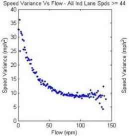
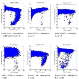
(12) 12. Theoretical framework. unreliable. 𝑣 𝛽 𝑇 = 𝑇 0 �1 + 𝛼 � � � 𝑐. (2.3). Instead of finding a direct relation between flow and speed, finding a relation between speed variance and flow could be an intermediate step. Blandin, Salam, and Bayen (2011) have researched this relation and found results as displayed in figure 2.2. In general it was found that higher flows lead to lower speed variances. These speed variances are measured per individual vehicle, under stationary conditions. In the research of Bulteau, Leblanc, Blandin, and Bayen (2012), however, a positive relation between those two variables was found. This positive relation is caused by the differences in speed between lanes. Those findings mean that under certain conditions, it is possible to say something about flow, when knowing the variance in speed and vice versa .. Figure 2.2: Relation between flow and speed variance (Blandin et al., 2011) A better relation was found by Blandin et al. (2011) between speed and flow directly. Some examples are shown in figure 2.3. Certain relations between the two variables can be seen here, in the form the fundamental diagram also has (figure 2.1). But this form is not always the same and often it is unclear where the separation between the free flow and the congested regime is situated. The duality of some of the intensities (it is unclear whether an intensity belongs to the free flow or the congested regime) is not fully clarified by these relations. Making estimations of speed, based on flow data have often been carried out by researches that do this based on single loop detectors (Coifman, 2001; Coifman & Kim, 2009). Making assumptions on or calculations of vehicle lengths is the base of these estimations. Jain and Coifman (2003) have conducted a research that is not based on this fact, but uses traffic flow theory principles to identify erroneous speed estimates. In this research data from adjacent lanes is combined to improve and filter bad estimations. This led to a significant improvement in speed estimations. Also research was done on estimating flow, based on knowledge of speeds. Altintasi, Tuydes-Yaman, and Tuncay (2017) find that even though having only average travel speed information, it is still possible to detect critical patterns on urban roads. Those patterns were not real flows, but it were states as ‘free flow’, or ‘dissolving congestion’ etc. Seo et al. (2017) state that without additional assumptions it is not possible to derive traffic state from only knowing speed (from floating car data). Always a fundamental diagram is needed for estimation, that needs to be calibrated on stationary data (Seo et al., 2017). Those researches show that under conditions it is possible to make estimations of speed based on flow data and vice versa. A very clear relation between those two traffic state defining variables, however, cannot be shown, there is always additional data needed to say something about its relation. The main difficulty in estimation is caused by the duality from the fundamental diagram in the speed flow relation..

(13) Machine learning in traffic engineering. 13. Figure 2.3: Relation between flow and speed (Blandin et al., 2011). 2.2 Machine learning in traffic engineering Machine learning algorithms can be used for numerous different tasks. The most well known example for this is image recognition. In this case an image is shown to the computer and the computer will recognise the object. But its applications are much broader than image recognition. In this chapter some well known machine learning techniques are discussed. Also the application of machine learning in the field of traffic engineering is discussed. 2.2.1 Regression Before discussing machine learning techniques, the principles of regression are discussed, since regression is more or less a basis of machine learning. In regression, input variables are taken to predict an output variable, based on known examples (a training set). In contrast to machine learning, which is a black box, regression uses mathematical functions in order to make a proper prediction on a certain output variable. Regression works by finding a function ℎ𝜃 (𝑥) that comes closest to the values 𝑦 of the training set. When 𝑦 is only dependent on one variable 𝑥, a cost function 𝐽 can be defined, based on the function ℎ𝜃 (𝑥(𝑖) ) = 𝜃0 + 𝜃1 𝑥(𝑖) . This cost function for 𝑚 samples is given in equation 2.4 (Ng, 2018). This cost function equals the mean squared error (MSE) between the estimated set and the set of the real values. Minimization of the cost function 𝐽(𝜃0 , 𝜃1 ) will find the values for 𝜃 that makes the best possible predictor for 𝑦, based on this regression technique. The cost function can be minimized using the method of gradient descent, which is discussed in chapter 2.2.3 on artificial neural networks. 𝐽(𝜃0 , 𝜃1 ) =. 1 𝑚 �(ℎ (𝑥(𝑖) ) − 𝑦(𝑖) )2 2𝑚 𝑖=1 𝜃. (2.4). Often 𝑦 is not dependent on only one variable, but there are multiple variables involved. The function ℎ𝜃 (𝑥) that describes 𝑦 in this case can be written as in equation 2.5 (Ng, 2018), in which 𝑥0 = 1 for the convenience of writing it vectorized. To find the values for 𝜃 the algorithm in equation 2.6 can be used for all features 𝑗 of the regression model. In this algorithm 𝛼 is the step size for the convergence of the model (Ng, 2018)..

(14) 14. Theoretical framework. ℎ𝜃 (𝑥) = 𝜃0 + 𝜃1 𝑥1 + ⋯ + 𝜃𝑛 𝑥𝑛 ⎡ ⎤ ⎢⎢𝑥0 ⎥⎥ ⎢⎢𝑥 ⎥⎥ = �𝜃0 𝜃1 ⋯ 𝜃𝑛 � ⎢⎢⎢ 1 ⎥⎥⎥ = 𝜃𝑇 𝑥 ⎢⎢ ⋮ ⎥⎥ ⎣ ⎦ 𝑥𝑛. (2.5). repeat until convergence: { 𝜃𝑗 ∶= 𝜃𝑗 − 𝛼. 𝑚. 1 �(ℎ𝜃 (𝑥(𝑖) ) − 𝑦(𝑖) ) ⋅ 𝑥(𝑖) 𝑗 𝑚 𝑖=1. for j := 0 ... n. (2.6). } The difference between regression and other machine learning techniques is that with regression the classification of data is based on mathematical rules and formulas. While with machine learning, the algorithm learns by example, instead of by rules. This makes that regression can be used for problems in which correlation can be easily found. In other cases, for example when it is not clear why a certain correlation is caused, or when the most accurate prediction possible are desired, machine learning techniques are a good alternative (Stewart, 2019). 2.2.2 Decision tree algorithms A decision tree is a model for supervised learning, in which the local region is identified in a sequence of splits (Alpaydin, 2010). The model is made of decision nodes in which a certain property is tested and dependent on the outcome a different path is chosen. By doing this all data is split into categories that will be identified by going through all steps. A simple example can be seen in figure 2.4. For each decision that is to be made a boundary needs to be found between two classifications. The main strategy that is followed by a decision tree algorithm is ‘divide-and-conquer’, this means that the problem is divided by the nodes in the tree, and it is attempted to make the division in each step as big as possible, in order to reduce the amount of decision nodes.. Figure 2.4: Decision tree in which the boundaries are shown as lines and the classifications as shapes (Alpaydin, 2010).. Decision trees are often used for classification problems. Advantages of decision tree models to more complex models, which may be more accurate, is that the model is very interpretable. The model can be written as a set of if-then rules and can be relatively easily understood by humans with knowledge in the field of application (Alpaydin, 2010). 2.2.3 Artificial Neural networks (ANN) A machine learning algorithm that is widely studied is the artificial neural network. Those neural networks consist of at least three components, which are the inputs, the hidden units and the outputs (Nielsen, 2017). Those three components can be regarded as layers of units, in which all units from each layer communicate with all units from all adjacent layers. In figure 2.5 a basic neural network is shown..

(15) Machine learning in traffic engineering. 15. hidden units. xD. (1) wMD. zM wK(2)M yK outputs. inputs. y1. x1 x0. z1. (2) w10. z0 Figure 2.5: A simple neural network with one hidden layer (Bishop, 2006). In a neural network, the nodes are called the neurons and can take any value between 0 and 1. All connections between the layers are weighted and so the value of the neurons in the next layer can be determined. The output of the neuron is determined by an activation function, often the sigmoid function (as can be seen in equation 2.7) is used for this. The 𝑧 in this function is a linear combination of all inputs and a bias and can be denoted as ∑𝑗 𝑊𝑗 𝑋𝑗 , in which 𝑋 represent the inputs (and the bias 𝑋0 , which always takes a value of 1) and 𝑊 the weights (Nielsen, 2017). The reason that the sigmoid function is applied is to scale the output to values between 0 and 1. Another scaling function that is often used is tanh (𝑧) which scales between -1 and 1. 𝜎(𝑧) =. 1 1 + 𝑒−𝑧. (2.7). As stated, the values for 𝑧 are determined by a linear combination. An example of this in matrix notation can be seen in equation 2.8 for the first step from the inputs 𝑋1 ...𝑋𝐷 to the hidden layer 𝑍1 ...𝑍𝑀 . A similar transition is made in the step between the hidden layer 𝑍1 ...𝑍𝑀 to the output layer 𝑌1 ...𝑌𝐾 . In these neural networks the first layer of neurons represent the inputs of the neural network (which is shown as 𝑋1 ...𝑋𝐷 in figure 2.5, 𝑋0 denotes the bias). In image recognition for example, every neuron in this network could represent the darkness of one pixel on a scale from 0 to 1. But in traffic engineering other inputs features can be given, such as present or past intensities together with the properties of the road. (1) ⎡ ⎤ ⎡ (1) ⎢⎢ 𝑍1 ⎥⎥ ⎢⎢⎢ 𝑊10 𝑊11 ⎢⎢ 𝑍 ⎥⎥ ⎢⎢ 𝑊 (1) 𝑊 (1) ⎢⎢ 2 ⎥⎥ = ⎢⎢ 20 21 ⎢⎢ ⋮ ⎥⎥ ⎢⎢ ⋮ ⋮ ⎢⎣ ⎥⎦ ⎢⎢ ⎣ (1) (1) 𝑍𝑀 𝑊𝑀0 𝑊𝑀1. (1) ⎤ ⎡ ⎤ … 𝑊1𝐷 ⎥⎥ ⎢ 𝑋0 ⎥ ⎢⎢ ⎥⎥ (1) ⎥ ⎥ … 𝑊2𝐷 ⎥⎥⎥ ⎢⎢⎢ 𝑋1 ⎥⎥⎥ ⋱ ⋮ ⎥⎥⎥⎥ ⎢⎢⎢⎣ ⋮ ⎥⎥⎥⎦ (1) ⎦ … 𝑊𝑀𝐷 𝑋𝐷. (2.8). The output layer (𝑌1 ...𝑌𝐾 in figure 2.5) provides the information that is requested. In the situation of traffic state estimation using intensity data this would be either a binary classification such as ‘free flow’ or ‘congested’, but it could also be more specific such as a real speed, or a range within the speed is expected to be. The output layer can be seen as a vector, in which all entries represent a classification. The number this vector entry (output neuron) holds, can be seen as a probability that given the input this classification would be correct. Between the input and the output layer, there is the hidden layer. This layer is called the hidden layer since it will never be completely clear what the values these neurons hold exactly mean. However, behaviour of single neurons can be studied and some logical patterns may be found. In this way it may be cleared up what the hidden layer ‘thinks’, when it is trained..

(16) 16. Theoretical framework. The properties of a neural network are defined by the weight matrices. Finding good values for these weights is done by training the network. In order to do this all weights are initiated randomly and after this gradually improved, until satisfactory weights are found. This is done by trying to minimize the error function. This error function gives the distance between the model output and the known answers from the training set. In equation 2.9 an error function is given (Bishop, 2006) for a training set of size 𝑛. In this function 𝑡 𝑛 stands for the target vector. 𝑁. 𝑤) = � 𝐸𝑛 (𝑤 𝑤) = 𝐸(𝑤 𝑛=1. 1 𝑁 � ||𝑦𝑦(𝑥𝑥𝑛 , 𝑤 ) − 𝑡 𝑛 ||2 2 𝑛=1. (2.9). This error function is often minimized with the method of gradient descent (Nielsen, 2017). With this 𝑤) smaller. This updating of weights takes place method the weights are updated in order to make 𝐸(𝑤 𝑤(𝜏) a weight vector as in equation 2.10 (Bishop, 2006), in which 𝜏 denotes the iteration step and Δ𝑤 𝑤). 𝜂 update, which in case of gradient descent is given by the gradient vector of the error function ∇𝐸(𝑤 is the learning rate of the method. 𝑤(𝜏) = 𝑤 (𝜏) − 𝜂∇𝐸(𝑤 𝑤(𝜏) ) 𝑤 (𝜏+1) = 𝑤 (𝜏) + Δ𝑤. (2.10). 𝑤) needs to be determined. For the network shown in figure To find the updated weights 𝑤 (𝜏+1) , ∇𝐸(𝑤 2.5, it can be found that 𝜕𝐸𝑛 𝜕𝐸𝑛 = 𝛿𝑘 𝑧𝑗 and = 𝛿𝑗 𝑥𝑖 (2.11) (2) (1) 𝜕𝑤𝑘𝑗 𝜕𝑤𝑗𝑖 in which. 𝐾. 𝛿𝑘 = 𝑦𝑘 − 𝑡𝑘 and 𝛿𝑗 = (1 − 𝑧2𝑗 ) � 𝑤𝑘𝑗 𝛿𝑘 .. (2.12). 𝑘=1. By iteratively updating the weights, by calculating the gradient of the error function, using the updated weights, a satisfactory low value for the error function may be found in a local minimum of the error function. It is hard, or often impossible, to claim whether or not a local minimum is the global minimum. Therefore it may be useful to repeat the procedure with different initial – random – weights, since different local minima may be found. Although the method of gradient descent is commonly used, also other optimization methods are available as the Levenberg-Marquardt method and the Genetic algorithm (Ma, Tao, Wang, Yu, & Wang, 2015). The main differences between machine learning methods such as decision tree algorithms and neural networks is that within decision trees it is relatively simple to see what happens in the model, while a neural network is more a ‘black box’ model, in which the algorithm learns by non-visible iterative steps. As it is easy to see how the decisions which are made within a decision tree algorithm separates different classes, it may be very difficult to find a proper decision tree when patterns within the available data are hard to find. In artificial neural networks, logical patterns do not need to be the input to the model in order to make a classification of the data. The neural network iteratively optimizes its result for the given training data. This makes it a good method for classifying data in which patterns cannot be found or are very hard to identify. However, sometimes ANNs give good results on training data, because it optimizes for this, but fails to do so on other data. 2.2.4 Deep neural networks (DNN) The difference between a ‘normal’ neural network and a deep neural network is the amount of hidden layers. In a conventional neural network there is only one hidden layer and only the amount of neurons is variable. In a deep neural network there are multiple hidden layers. This can range from a few hidden layers to over a hundred (MathWorks, 2017). In figure 2.6 the architecture of a deep neural network is shown..

(17) 17. Inputs. Ouputs. Machine learning in traffic engineering. Input Layer. Hidden Layers. Output Layer. Figure 2.6: A deep neural network with multiple layers (MathWorks, 2017) Advantages of deep learning networks compared to normal neural networks are improved accuracy of predictions made. Since there are many more connections to be made when there are more layers present. At the same time the large number of connections in a neural network has some disadvantages. In the first place it will take much longer to train the network. The fine-tuning of weights is the method to train the network, so with many more weights this fine-tuning will take much more time. Since deep neural networks are more sophisticated than normal neural networks because of the higher amount of hidden layers, it can be trained so that for the training and the test data it will give very accurate results. However, this does not automatically mean that the network is of good quality. When the amount of connections is much higher than the amount really needed, the ‘training’ of the network will at some point become optimized for the provided data, instead of finding patterns that can be applied to other cases. So it will always be needed to evaluate the complexity of the network that is needed for the particular problem. 2.2.5 Recurrent neural networks (RNN) Another variant on the neural network is the recurrent neural network (RNN). In this network the input is not only fed forward, but feedback loops are included, an example of such a network can be seen in figure 2.7.. Hidden layer. Ouput layer. Outputs. Inputs. Input layer. Figure 2.7: A recurrent neural network, in which the output layer is fed back to the hidden layer (Quiza & Davim, 2009). In an ordinary neural network all inputs are sent through the network at once, so a single output is given. In a RNN time plays a role and the output is not determined instantly but with time steps. In every next step the output of the network will be fed back to the hidden layer. In this way with every next time step the output will change (Nielsen, 2017). RNNs are good for the capturing evolution of traffic flow, volume and speed. Since RNNs use internal memory units for processing arbitrary sequences of inputs, RNNs have the capability of learning temporal sequence (Ma et al., 2015). Traffic patterns are defined by temporal sequences of the traffic.

(18) 18. Theoretical framework. state variables, therefore RNNs are expected to capture patterns in a better way than ordinary ANNs. 2.2.6 Use for traffic state estimation Several researches have been conducted on using big data / machine learning in traffic engineering. Most of these researches are about traffic flow prediction, but there are also some papers on traffic state estimation. Giving this short overview will help to see what techniques were found useful for which application in traffic engineering. Most of the applications of machine learning within the field of traffic engineering are about forecasting the near feature, based on current traffic variables. Good results have been found by using (deep) neural networks for the short term prediction on traffic flow (Polson & Sokolov, 2017; Zhu, Cao, & Zhu, 2014) and using several machine learning techniques on short term prediction of traffic speed (Ma et al., 2015; Fusco, Colombaroni, & Isaenko, 2016). The challenge for this research, however, is not to make a forecast of traffic state, but to define traffic state when only one of the defining variables is available. DatMobility (2017) has conducted a research on using an ANN to make an estimation of whether or not there is congestion, based on 15 minute aggregate data of modelled traffic flow. The input for this model intensity data was used. These intensities are from the road stretch for which the classification is made, as well from the road stretch upstream and downstream. The intensities that are used are the intensity of the moment for which the state of congestion is estimated and three data points of 15 minute aggregate intensity before that. So for the input intensities variation was made both in time and space. The research showed rather good results on the training set, but for other situations it mostly failed to detect congestion, so likely the ANN that was used was trained for the specific situation, in stead of being a generic model. This could have been caused by model overfitting, but it is more likely that there were characteristics of the specific road situations that were not included in the model. It is hard to say which characteristics this were exactly, but missing those makes that a model trained one road situation is not transferable to other locations. 2.2.7 Comparison of techniques Regression is a non-machine learning mathematical approach for classifying data based on mathematical rules, while machine learning techniques learn by example and are therefore useful when a clear relation between input variables and the classification cannot be found. Within machine learning, two methods are decision tree learning and artificial neural networks. DTL divides the data into categories and by doing this a tree with branches and leaves is constructed. ANNs take input data and process it through hidden layers of neurons, in order to make a prediction of a specified category. Variants on the ANN are the deep neural network and the recurrent neural network. The advantages of such more complex networks is that its results are often more accurate. RNNs can be useful when changes during time are important for the classification of data. Drawbacks of these more complex techniques are more calculation time and that it may become harder to correctly interpret the results. When using DTL techniques it is very clear what the output of the machine learning is. It will be a set of rules on which decisions are made, that makes it useful for finding how the input variables are used within the model. RNNs are made for situations when patterns in time series are to be found, which is the case when classifying speeds base on intensity series. Because of the properties of these techniques it is chosen to apply these in the research..

(19) 3 Methodology The approach that is used in order to be able to answer the research question is discussed in this chapter. Since the final aim of this research is to come up with a model that is able to estimate traffic state from intensity data, all steps that are taken will serve this goal. The following steps will be taken: 1. Collection of data; 2. Testing different kind of models; 3. Testing additional input attributes; 4. Testing multiple roads. This methodology explains how those steps are taken.. 3.1 Data collection 3.1.1 Data selection and gathering In order to research the relation between intensity and speed patterns on highways using machine learning techniques, data needs to be acquired. This needs to be highway data where speed is linked to flow, in order to train a supervised machine learning model. Also this data should be diverse in terms of road properties, because otherwise the model could train for one specific situation. Within this data locations in which congestion occurs have to be included. For the road stretches the data is acquired from the ‘Nationale Databank Wegverkeergegevens’ (NDW, 2018), which has a tool for downloading historical highway data on a one minute time resolution. The definition for road stretch will be derived from this NDW data. A road stretch or a road section is defined as the road around a detection loop. The beginning of this section is the upstream detection loop and the end the downstream detection loop. Using NDW data means that the model is trained on measured intensities and not on modelled intensities, which is a use case for this research. But it is assumed that it is better to train a model based on measured intensity and measured speed data, than when modelled intensity data is linked to measured speeds. For doing this research twelve locations are selected, that have a certain diversity on road characteristics. Most locations need to have an identifiable bottleneck, because these locations are expected to have the properties to make good estimations. Also locations without a bottleneck are included. All those locations need to have detection loop data available on its location, as well upstream and downstream from the location. For the researched location speed information must be available, for the upstream and downstream location intensity is enough. In this research, complex road situations, such as weaving lanes at motorway intersections, peak lanes, motorways where transit traffic are separated from local traffic and other complex situations, other than lane drops and ramps, are not included in this research. Those situations are hard to fit in the model because of their specific characteristics. Using the format in this research where only intensities are used from the location (and upstream and downstream), would not be possible. Testing the different types of machine learning models is done on a selected road section that has a very clear bottleneck, so good estimation can be made on the traffic state. Also for testing which additional properties, a location with a clear bottleneck is selected. This location must have information on vehicle length available, because this is one of the additional properties that the road is tested on.. 19.

(20) 20. Methodology. For the selection of the road stretches a diversity is pursued. This means those road stretches will differ in the number of lanes, their place in the network, whether or not on– and off ramps are present, being upstream or downstream of a bottleneck and speed limit. This diversity will be in both the training and the testing data. For all road stretches both speed and intensity have to be known, as well for the researched road stretch as the road stretches up– an downstream. Not all this data can be acquired by NDW, but Google Maps is used to gain additional information. Other properties of the researched road stretches that are needed are the speed limit at the time, whether or not an on– or off ramp is present, the number of lanes and for the up– and downstream road stretch, the distance to the researched road stretch and whether or not there is a lane drop. All those features are listed in table 3.1. These properties are included because they are the main characteristics of the road. These properties will vary for each road section, so information on these properties is needed to identify the type of road. Having all properties that define a road situation included in the model may make it possible to use another road section for testing and for training. Table 3.1: Input to machine learning model Selected road stretch Speed 𝑡0 Intensity 𝑡0 , 𝑡−1 , 𝑡+1 — Speed limit Number of lanes On-ramp lane present Off-ramp lane present Presence of lane drop. Upstream road stretch — Intensity 𝑡0 , 𝑡−1 , 𝑡+1 Distance to selected road stretch Speed limit Number of lanes On-ramp lane present Off-ramp lane present Presence of lane drop. Downstream road stretch — Intensity 𝑡0 , 𝑡−1 , 𝑡+1 Distance to selected road stretch Speed limit Number of lanes On-ramp lane present Off-ramp lane present Presence of lane drop. 3.1.2 Data preparation Applying machine learning techniques will be done by using weka. Weka is a software package that includes many different machine learning algorithms (University of Waikato, 2019). Algorithms that are included are regression methods, decision tree learning models and neural networks. Weka is originally a Java based program that can be used using a GUI or in Java. There is a Python API available (Python-weka-wrapper, 2019), that is used in the research to include the weka models in the other program code. The gathered data needs to be put in a form that it can be used by the weka software. But first the data needs to be aggregated in the way the data will be used. In order to be comparable to the research by DatMobility (2017), and to be applicable for comparable causes, it is chosen to aggregate the data to 15 minute data, because the modelled data that this research will be used for, also has a time resolution of 15 minutes. Since NDW highway data comes with a resolution of 1 minute, this has to be changed. For intensities this is relatively easy, since all intensities can be added to each other. The best way for aggregating speed is calculating the space mean speed. This is not as straightforward as calculating the time mean speed, which is just a weighted average of all the speeds of every one minute data interval of the vehicles that pass. A way for finding the space mean speed is shown in equation 3.1 (Soriguera & Robusté, 2011). This will be applied in aggregating the speed data from one minute to 15 minute intervals. It has to be noted that the original one minute aggregate data consists of time mean speeds, this cannot be changed to space mean speeds. This means that the 15 minute aggregate speed value is not the true space mean speed, but an approximation of the space mean speed. 𝑣𝑠 = 𝑣𝑡 −. 𝜎2𝑡 𝑣𝑡. (3.1).

(21) Testing several models. 21. Whenever an erroneous data entry is found, it is removed from the dataset if it is possible to still keep reliable data. This means that when for one aggregated 15 minute data point for example one minute of a certain vehicle category is missing, the data point can still be determined in a reliable way, since most data is available. In the case many data are missing or corrupted it is considered to delete that certain day for that certain road stretch from the dataset, since it may influence the model too much. If this is the case another day will replace this day of data, this will be a day that is the same day of the week and close to the original day that was used in the model. If structural errors or missing data is found for a certain road stretch, it is decided to replace this road stretch with a similar road stretch, that has no structural errors in the data.. 3.2 Testing several models When the data is prepared in the format that is needed for weka, the models are trained. It is chosen to train both a decision tree learning model (DTL) and a recurrent neural network (RNN). But before training these machine learning models a regression model is applied, in order to see the performance of linear regression. The DTL model can be useful, because it can give a good insight in what happens in the model, because this will divide characteristics into branches and leaves. Also it has not been tested yet for this particular problem. RNNs are good in working with time series, and will probably give in this situation better results than ANNs, which are tested in the research of DatMobility (2017). Since these models are only applied to one single road stretch, the speed limit, number of lanes and the prevalence of ramps will be constant on this road section, therefore they will not be included as an input to the model. The input that remains is the intensity data of the researched road stretch, the intensities up– and downstream and the distances to this up– and downstream locations. For testing the additional input attributes, these attributes are added to the intensities. For congestion estimation multiple performance measures can be used. The most simple measure is the accuracy, which simply gives the percentage of correctly identified instances. A disadvantage of this measure is that in cases with a low number of congested instances, identifying all instances as not congested will lead to a very high accuracy. That is why it is chosen not to use accuracy as a performance measure. The measure that is used in this research is the f-score, which can be seen in equation 3.2. The f-score is a compromise between precision and recall. The precision is the share of correctly identified cases of congestion of the total number of congestion identifications. The recall is the share of correctly identified cases of congestion of the total number of cases of congestion. These two measures include the number of false positives and false negatives. The f-score gives a better view on whether or not the model is able to capture congestion than precision and recall separately. ⎛ ⎞−1 ⎜⎜ precision−1 + recall−1 ⎟⎟ precision ⋅ recall ⎟⎠ = 2 ⋅ F1 = ⎜⎝ 2 precision + recall. (3.2). For estimating speed the root mean squared error (RMSE) is the performance measure that is used (equation 3.3, in which 𝑌̂ are the estimated speed values and 𝑌 the measured speeds). Other measures are available, such as the MASE (mean absolute scaled error), which just calculates the average of all errors. The advantage of the RMSE is that it gives a larger penalty to larger errors. This is useful in the researched situation, since the data can be roughly divided into congestion and free flow and having a larger penalty for larger errors, gives a big punishment for estimated speeds that are free flow and are estimated congested and vice versa.. 𝑅𝑀𝑆𝐸 = �. 1 𝑛 �(𝑌 − 𝑌̂ 𝑖 )2 𝑛 𝑖=1 𝑖. (3.3).

(22) 22. Methodology. The model that is found to have the best results is used for the other parts of this research. Because it is expected that this model will also be best fitted for all other uses of the model, such as attribute testing. The best model will be validated by testing on the other road sections.. 3.3 Testing additional attributes In order to improve the results of the testing on a single road stretch, the influence of additional attributes is tested. These attributes are added to the intensities that originally were the only input to the model. A road section is selected for carrying out those tests. The following three attributes are tested: 1. Weather information; 2. Percentage of long vehicles; 3. Deviation in the intensity data. For information on the weather KNMI data is used from a nearby station. KNMI has data on whether or not bad weather circumstances have occurred during a certain period. For most locations there is information available on the share of long vehicles, this data can be acquired from the NDW data. The last value that is tested is the deviation in intensity data. Because all data was aggregated to 15 minute intervals from one minute intervals, it is possible to calculate the standard deviation of the intensity of these intervals. This deviation can be an indication of changing circumstances. Whether or not these three factor have influence is tested by comparing the f-scores and RMSEs to the base test, where only intensities are fed to the model. If a positive change is registered, this additional attribute can be of extra value to the model. The attributes that contribute positively to the model are also combined and tested. The best configuration found will be validated on the other road sections.. 3.4 Testing on a set of multiple roads At first the machine learning models were trained for the researched road stretches only, this means all selected road stretches are trained individually and tested individually. Now a general classification model will be made. In contrary to the previous part of the research, where only one road stretch was researched, now different road stretches together will serve as an input to the model. This means that also a variety in road properties is introduced at this point. So from this point onwards the speed limit, the amount of lanes and the prevalence of ramps are used as an input. Also intensities are normalized, in order to make them comparable to each other. This has been done by representing intensities as a percentage of the roads capacity. This capacity is determined by the value in which 99% of all values on that road are lower than the capacity value. This part of the research consists of two parts. In the first part all road sections are combined in one training set and tested on each road individually. This makes it possible to see if adding multiple roads as an input confuses the model, or whether it is still possible to make proper estimations. The results of this testing are compared to the results of testing on models that are trained on one specific road. In the second part the models will be tested on roads that are not included in the train set. This must show if it is possible that properties of the roads are transferable to other roads, so still good results can be found. Also here the finding are compared to the results of specific road testing..

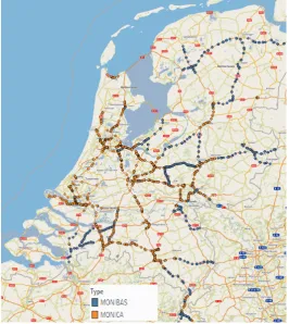
(23) 4 Data collection The data that is used to train a speed estimation model contains data of both traffic speed and intensity. In this chapter it is discussed which data is obtained, how it is processed and what are the properties of the data.. 4.1 Data Sources Two main sources for traffic analysis are available, which are loop detector data and floating car data. Since for floating car data a good estimation of speed can be made, but it is very hard to give a good indication of traffic flow, detector data is the preferable data source to use for this research and this is used for this research. 4.1.1 MoniCa / MoniBas In the Netherlands many highways are equipped with the MoniCa detector system, which is a double loop detector in the road that is able to measure both speed and intensities. MoniBas is the name for the processed data from MoniCa. MoniBas checks the MoniCa data for reliability and missing data (De Jong, 2012). NDW (Nationale Databank Wegverkeergegevens) is a corporation of several administrations in the Netherlands, such as provinces and Rijkswaterstaat. NDW gathers, manages and distributes traffic data in the Netherlands, that can be used for traffic information and traffic studies. It also makes detector data for the roads in the Netherlands available. MoniBas data, and also raw MoniCa data at some places is available in this data set. This dataset is the data source that is used for this research.. Figure 4.1: MoniCa and MoniBas locations where the data is divided into vehicle classes.. 23.

(24) 24. Data collection. 4.1.2 Characteristics of the data All MoniCa and MoniBas data from NDW contain information on both intensities and speeds. This is available for each individual lane in one minute intervals. Some of the MoniBas data makes a distinction between different vehicle classes, also the raw MoniCa data does this. All passing vehicles are divided into three length categories (which can be found in table 4.4). This distinction can be used to see differences in speed between different vehicle classes or can be used to determine the percentage of long vehicles. This share of long vehicles is a property that is researched. Not all MoniBas data makes this vehicle length distinction, many data entries only provide the class ‘anyVehicle’, in which all lengths are aggregated. In figure 4.1 it is shown at which locations in the Netherlands MoniCa and MoniBas data is available that have the different vehicle classes, these are the best locations for using in this research. 4.1.3 Data completion When a minute of data is missing or corrupt, MoniBas completes the data if the duration of the missing data is not more than 5 minutes. Within the MoniBas system there is a check for whether or not data is correct. Sometimes the vehicle categories are only available in the MoniCa data and not in the MoniBas data. In this case MoniCa data is used and processed in a way that is is usable, such as the MoniBas data. Whenever there is corrupt of missing data, a gap within the time line of data points evolves. MoniBas does fill in the values of this gap, if the length of the gap is not more than 5 minutes. For completing the data the last accepted minute value (𝑡1 ) from before the gap of missing data and the first accepted minute value (𝑡2 ) from after the gap are used. For the minutes in between (never more than 5), the value for intensity (𝐼) or the speed (here defined as 1/𝑣) are chosen on the linear interval between the values of 𝑡1 and 𝑡2 , as can be seen in figure 4.2 and in equations 4.1 and 4.2 (NDW, 2013). Whenever MoniCa data is used and data is missing, the same rules as for completion of the MoniBas data are applied. 𝐼𝑡 = 𝐼𝑡1 + (𝑡 − 𝑡1 ). 𝐼𝑡2 − 𝐼𝑡1. (4.1). 𝑡2 − 𝑡 1. 1/𝑣𝑡2 − 1/𝑣𝑡1 1 1 = + (𝑡 − 𝑡1 ) 𝑣𝑡 𝑣𝑡1 𝑡2 − 𝑡 1. (4.2). I or 1/v. In which 𝐼𝑡 is the interpolated value for intensity and 𝑣𝑡 the interpolated value for speed. 𝑡1 indicates the time of the last known value before the gap and 𝑡2 the time of the first correct value after the gap. This interpolation is applied for all minutes within the gap, making the time series complete again.. t1. t. t2. Figure 4.2: Completion of missing data in MoniBas. The blue points indicate normal data points in the dataset,. the gap between 𝑡1 and 𝑡2 that came from missing or corrupt data is filled with interpolation, based on the last value before and the first value after the gap. When the gap is no longer than 5 minutes, this results into a continuing stream of data points..

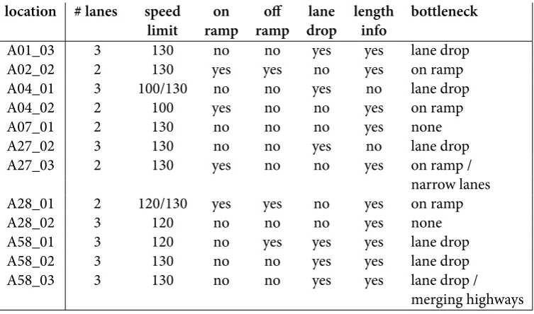
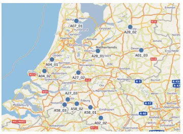
(25) 25. Locations. 4.2 Locations A total of twelve locations have been selected for this research. These locations cover different kind of road situations. Most of these road situations are bottlenecks, but also situations without bottlenecks are researched. Different kind of road section have been researched, because the goal is to create a model that can estimate speeds on a wide range of locations The reason that many bottlenecks are researched, is that at these locations the relation between intensity and speed is expected to be most easily demonstrated. At a bottleneck it is most times very clear what is the cause of congestion and congestion will occur regularly. Especially lane drops are bottlenecks that can well be fit into models, because in contrary to ramps, all traffic stays on the same road, there is no traffic leaving or entering the road. In table 4.1 an overview is given of the locations, which are put on a map in figure 4.3. As can be seen six of the selected location contain a lane drop. four have an on-ramp and two have no particular bottlenecks. Most locations have information available on the length of the vehicles, just two do not. One location on the A27 near Breda is located on a bridge, which causes the lanes to be more narrow than normal lanes, which may be regarded as a flow preserving bottleneck. Another case that is unique in these locations is the A58 near Breda, where two motorways are merging. This can be seen as an ordinary lane drop, but upstream there is not one road, but there are two different roads. Table 4.1: Specifications of the locations in this research. location. # lanes 3 2 3 2 2 3 2. speed limit 130 130 100/130 100 130 130 130. on ramp no yes no yes no no yes. off ramp no yes no no no no no. lane drop yes no yes no no yes no. length info yes yes no yes yes no yes. A01_03 A02_02 A04_01 A04_02 A07_01 A27_02 A27_03 A28_01 A28_02 A58_01 A58_02 A58_03. 2 3 3 3 3. 120/130 120 120 130 130. yes no no no no. yes no yes no no. no no yes yes yes. yes yes yes yes yes. bottleneck lane drop on ramp lane drop on ramp none lane drop on ramp / narrow lanes on ramp none lane drop lane drop lane drop / merging highways. 4.3 Time periods Three time periods of three weeks are selected to use as input data for the model. These three periods are chosen throughout the year, so not only one single season is researched. From all three periods the first two weeks will serve as training data for the model and the last week as testing data, so all periods have both training and testing data. In table 4.2 the three periods are shown. Taking this time span of nine weeks creates 6048 instances per road of which two third is used for training, the other third for testing purposes. For two days (5 and 10 October 2017) there was much missing data for all points. Therefore it was chosen to replace these days with two other comparable days. Both days were replaced by the same day of the week of the week after the October period. A day that is included in the data set, that was remarkable, is 18 January 2018. On that day on many measurement locations low speeds were registered. This was caused by a severe storm in the Netherlands,.

(26) 26. Data collection. Figure 4.3: The twelve locations that are used in this research. Table 4.2: Time periods in which is measured. 1 2 3. training set begin 01-10-2017 07-01-2018 01-04-2018. end 14-10-2017 20-01-2018 14-04-2018. test set begin 15-10-2017 21-01-2018 15-04-2018. end 21-10-2017 27-01-2018 21-04-2018. in which was advised not to drive (code red). In the chosen road sections however, no special congestion due to this fact was found and therefore it is chosen to keep this day in the dataset. It is chosen not to exclude non-recurring traffic patterns. It may be argued that having only regular situation in the dataset makes better predictions possible, but excluding this data makes that this model can only identify recurrent patterns. When this data is included, the model can be trained on situations that do not often occur. Having this data included in the data increases its estimating power. Also it will probably not lead to confusion in the training set, as there will be enough examples of recurring congestion. This means that not excluding special event data will lead to the same capabilities as when they would be excluded, but including makes that the model has a higher change of also capturing special event situations.. 4.4 Obtaining and processing the data The data is obtained by making requests at NDW (Nationale Databank Wegverkeergegevens) for the selected time periods. The data was made available in large XML-files that contain all measurement points of the Netherlands. These XML files were parsed using a Python script and the selected locations – together with some upstream and downstream measurement points – were filtered out of this data and stored to a plain text format, which makes is easy to access the data when needed. Since the NDW data comes at a time resolution of one minute, it was aggregated to 15 minute intervals, because that time resolution was chosen for this research. This was also done using a python script. For aggregating the intensity the values of all lanes and all separate minutes were added. This value is corrected, so the unit of intensity will remain veh/h..

No results found