NEW METHODS USING IN-SITU AND
REMOTE-SENSING OBSERVATIONS FOR
IMPROVED METEOROLOGICAL ANALYSIS
ERIK GREGOW CONTRIBUTIONS
142
No. 142
NEW METHODS USING IN-SITU AND REMOTE-SENSING OBSERVATIONS FOR IMPROVED METEOROLOGICAL ANALYSIS
Erik Gregow
Department of Physics Faculty of Science University of Helsinki
Helsinki, Finland
ACADEMIC DISSERTATIONin meteorology
To be presented, with the permission of the Faculty of Science of the University of Helsinki, for public criticism in E204 auditorium at Physicum (Gustaf Hällströmin katu 2 A, Helsinki) on February 9th, 2018, at 12 noon.
Finnish Meteorological Institute Helsinki, 2018
Finnish Meteorological Institute, Finland
Dr. Carl Fortelius
Meteorological Research, Numerical Weather Prediction Finnish Meteorological Institute, Finland
Reviewers Associate Professor Piia Post Institute of Physics
University of Tartu, Estonia
Dr. Niels Woetman Nielsen Centre for Meteorological Models
Danish Meteorological Institute, Denmark
Custos Professor Heikki Järvinen
Department of Physics University of Helsinki, Finland
Opponent Associate Professor Joan Bech
Department of Applied Physics - Meteorology University of Barcelona, Spain
ISBN 978-952-336-042-6 (paperback) ISBN 978-952-336-043-3 (pdf)
ISSN 0782-6117
Erweko Helsinki 2018
00101 Helsinki Date
February 2018
Author Erik Gregow Title
New methods using in-situ and remote-sensing observations for improved meteorological analysis Abstract
Observations have been and are an important part of today's meteorological developments. Surface observations are very useful as they are, providing weather information for a point location. ough they do not give much information, if any, on what happens between the stations across a larger area. With models one can create an analysis of the meteorological situation, i.e. calculate and estimate what happens between these fixed observation points. Remote-sensing data, such as radar and satellite, are being processed and the output is given over a domain as an analysed product of their measurements. For example, radar gives a plot of where the rain is located, i.e. an analysis of the current precipitation.
With a series of radar images, a human (subjectively) or a computer (objectively) can process this information to estimate where the rain will move and be located within the next few minutes (even hours), i.e. a short forecast also called "nowcast". is applies to some extent also for other observations, such as satellite data (cloud propagation). But for most quantities (such as temperature, wind, etc) it is significantly harder to make such a nowcast, since these are influenced by many other factors and there is no linear development of them. erefore, there are forecast models that solve physical and dynamic equations, so that one can estimate the future weather for the coming hours and days. A prerequisite for generating a forecast of high quality is to capture the initial weather conditions as best as possible. is is done using observations and they are introduced into the forecast model through different techniques, where the model creates its own analysis as the initial step. ere remain problems since forecast models oen are affected by physical disagreements, as the dynamic conditions are not in balance. is results in the model having a spin-up effect, where the meteorological quantities are not yet in balance with each other and the resulting weather conditions are not always reliable during the first hours. Hence, a lot of research is spent on how to reduce this spin-up effect and on the use of nowcast models, in order to deliver the best model results for the first few hours of the forecast period.
In this dissertation, the research work has been to improve the meteorological analysis, algorithms and functionality, using the Local Analysis and Prediction System (LAPS) model. Different kinds of observations were used and their interdependencies have been studied, in order to combine and merge information from various instruments. Primarily focus has been to improve the estimation of precipitation accumulation and meteorological quantities that affect wind energy. e LAPS developments have been used for several end-users and nowcasting applications, and experimentally as initial conditions for forecast modelling. e studies have been concentrated on Finland and nearby sea areas, with the available datasets for this domain.
By combining surface-station measurements, radar and lightning information, one can improve the precipitation-amount estimations. e use of lightning data further improves the estimates and gives the advantage of having additional data outside radar coverage, which can potentially be very useful for example over sea areas. In addition, the improved LAPS analyses (cloud-related quantities) and a newly developed model (LOWICE), calculating the electricity production during wintertime (taking into account the icing of wind turbine rotor blades which reduces efficiency), have shown good results.
Classification (UDC) Keywords
556.12, 551.508.85 Precipitation, observations, radar, lightning
.5 , . wind energy, wind-power, wind-turbine icing,
power-loss ISSN and series title
0782-6117 Finnish Meteorological Institute Contributions
ISBN Language Pages
ISBN 978-952-336-042-6 (paperback), English 106
978-952-336-043-3 (pdf) 621 48 624 143
00101 Helsinki Publicerat Februari 2018
Författare Erik Gregow Titel
Nya metoder för användande av observationer och förbättrade meteorologiska analyser Abstrakt
Observationer har varit och är en betydelsefull del i den meteorologiska utvecklingen. Markobservationer är mycket användbara som de är, de tillför väderdata för en specifik punkt. Men de ger ingen information om vad som händer mellan dessa mätpunkter. Med modeller kan man skapa en analys, dvs beräkna och estimera vad som händer mel-lan dessa observationstationer. Radar och satellit ger data över områden och är en produkt där dess mätningar är analyserade. Till exempel, radar ger en bild av var regnet befinner sig, dvs en analys av nuläget.
Med en serie av radar bilder, kan en människa (subjektivt) eller en dator (objektivt) bearbeta denna information så att man får en uppfattning om var regnet kommer att befinna sig inom de närmaste minuterna (även timmarna), dvs en kort progonos även kallat “nowcast”. Detta gäller även i stor utsträckning för övriga observationer, såsom satellit data (molnutbredning) etc. För meteorologiska parametrar såsom temperatur eller vind, är det dock betydligt svårare att göra en sådan nowcast, då dessa påverkas av många andra faktorer och det finns inte en linjär utveckling av dem. För att lösa detta problem finns det prognos-modeller, som löser de fysikaliska och dynamiska ekvationerna så att man kan få en bild av kommande väderparametrar för de kommande timmarna och dygnen. En förutsättning för en bra prognos är att man fångar det initiala väderläget så bra som möjligt. Detta görs med observationer och de introduceras i prognosmodellen via olika tekniker. Här kvarstår ett problem då modeller påverkas av fysikaliska oenigheter då de dynamiska förhållandena är i obalans. Detta resulterar oa i att modellen under de första timmarna har en “spin-up” effekt där de meteorologiska parametrarna ännu inte är i balans med varandra och de utvecklade väderförhållandena ännu inte är helt tillförlitliga. Därav spenderas mycket forskning om hur man kan reducera denna spin-up effekt och användandet av nowcast-modeller för att tillföra bästa modell resultat för de närmaste timmarna. I denna avhandling har fokus varit att förbättra den meteorologiska analysen (algoritmer och funktionalitet), genom att använda modellen Local Analysis and Prediction System (LAPS). Ett flertal observationer har använts och deras inbördes påverkan studerats, för att I bästa möjliga mån kombinera information från dessa olika instrument. Fokus har främst varit med avseende på nederbördsmängd och beräkning av meteorologiska parametrar som påver-kar vindkrasenergi. LAPS har även använts experimentellt i nowcasting sye och som analys för prognos-model, för att förbättra prognoserna i närtid. Studierna har i första hand fokuserat på Finland, med närliggande havsområden och tillhörande observations nätverk och instrumentering.
Vi har funnit att genom användandet av mark-stationer, radar och blixtnedslags information så kan man förbätt-ra bestämningen av nederbördsmängden. Användandet av blixtdata ger möjligheten att bestämma nederbörd över områden där det inte finns radar, till exempel över havsområden, vilket förr inte varit möjligt. Därtill har vi med förbättrade LAPS analyser (främst moln relaterade parametrar) och en nyutvecklad modell (LOWICE) påvisat posi-tiva resultat vid beräkning av elproduktionen under vintertid, där man tar i beaktning nedisning av vindkraverkens rotorblad, vilket sänker effektiviteten.
Klassficering (UDK) Sökord
556.12, 551.508.85 Observationer, nederbördsmängd, radar, blixtar
.5 , . Vindkra, vindenergi, nedisning
ISSN och serie titel
0782-6117 Finnish Meteorological Institute Contributions
ISBN Språk Antal sidor
ISBN 978-952-336-042-6 (paperback), Svenska 106
978-952-336-043-3 (pdf) 621 48 624 143
e work presented in this thesis has been carried out in the Meteorological Research Unit of the Finnish Meteorological Institute (FMI), while participating in several different projects and through involvement in many operational development works.
I thank all the co-authors and people who have helped me during this work.
I want to thank FMI for the opportunity to work among experts within the NWP field and including me in many interesting projects. I have always felt warmly welcome and there has been a positive spirit surrounding the cooperative work within the unit and whole of FMI.
I want to thank Professors Heikki Järvinen and Hannu Savijärvi for the support and help during my PhD work.
I want to express my deepest gratitude to Dr. Elena Saltikoff who has always been there to help, supervise and guide me, whenever in scientific troubles. Many thanks to Drs Carl Fortelius and Sami Niemelä who have been excellent supervisors during the years of my work at FMI and Docent Curtis Wood for helping in the final polishing of the thesis.
anks to specialist Ben Bernstein for helping with scientific questions and becoming a dear friend during the years of work together, thank you.
A special thank you to Professor Wahé Balekjian, who I have always looked up to and who encouraged me to study for this Doctorate. My thoughts go also to my mother Margareta, my Aunt Birgitta, my siblings and Annika who are, and always will be, the foundation in my life. Last, but not least, my children Anni and Nelli: You are my everything!
Erik Gregow
Acronyms - Abbreviations . . . 9
List of the original publications . . . 10
Summaries of the original publications . . . 11
1. Introduction . . . 14
2. Research motivations, questions and goals . . . 17
3. Methods and materials . . . 18
3.1. e Local Analysis and Prediction System (LAPS) . . . 19
3.1.1 LAPS – e RandB method . . . 20
3.1.2 LAPS – Lightning Data Assimilation (LDA) method . . . 21
3.1.3 LAPS – LOWICE method . . . 21
3.2. Observational datasets . . . 24
3.2.1 Surface gauges . . . 24
3.2.2 Radars . . . 25
3.2.3 Lightning-detection system . . . 26
3.2.4 Icing detection . . . 26
3.2.5 Wind-power production measurements . . . 27
4. Summary of the results . . . 28
4.1. Precipitation accumulation estimates . . . 28
4.2. Wind-power production and icing . . . 31
5. Discussion . . . 33
6. Conclusions . . . 36
3D – ree-Dimensional
AWS – Automatic Weather Station CBZ – Cloud-Base Height
CORR – Correlation
CRR – Convective Rainfall Rate DA – Data Assimilation
ECMWF – European Centre for Medium-Range Weather Forecasts FMI – Finnish Meteorological Institute
FTA – Finnish Transport Agency
HIRLAM – High Resolution Limited Area Model IFS – Integrated Forecasting System
INCA – Integrated Nowcasting through Comprehensive Analysis LAPS – Local Analysis and Prediction System
LDA – Lightning Data Assimilation LEA – Leading Edge Atmospherics LF – Low Frequency
LLS – Lightning-Location System LWC – Liquid Water Content MAE – Mean Absolute Error
MESAN – Mesoscale Analysis System MOS – Model Output Statistics
NORDLIS – Nordic Lightning-Information System NWP – Numerical Weather Prediction
PPI – Plan-Position Indicator PC – Precipitating Clouds QC – Quality Control
QPE – Quantitative Precipitation Estimation RandB – Regression and Barnes
RMSE – Root Mean Square Error
SLWC – Supercooled Liquid Water Content STDEV – Standard Deviation
STEPS – Short-Term Ensemble Prediction System VERA – Vienna Enhanced Resolution Analysis VHF – Very-High Frequency
I Gregow, E., E. Saltikoff, S. Albers, and H. Hohti, 2013: Precipitation accumulation analysis – assimilation of radar–gauge measurements and validation of different methods, Hydrol. Earth Syst. Sci., 17, 4109–4120, doi:10.5194/hess-17-4109-2013
II Gregow, E., B. Bernstein, I. Wittmeyer, and J. Hirvonen, 2015: LAPS-LOWICE: A Real-Time System for the Assessment of Low-Level Icing Conditions and eir Effect on Wind Power,J. Atmos. Oceanic Technol.,32(8), 1447–1463, doi: http://dx.doi.org/10.1175/JTECH-D-14-00151.1
III Gregow, E., A. Pessi, A. Mäkelä, and E. Saltikoff, 2017: Improving the precipitation accumulation analysis using lightning measurements and different integration periods, Hydrol. Earth Syst. Sci., 21, 267–279, doi:10.5194/hess-21-267-2017
IV Mäkelä, A., E. Saltikoff, J. Julkunen, I. Juga, E. Gregow, and S. Niemelä, 2013: Cold-season thunderstorms in Finland and their effect on aviation safety,Bull. Amer. Meteor. Soc.,94, 847–858, doi:10.1175/BAMS-D-12-00039.1
I.Gregow, E., E. Saltikoff, S. Albers, and H. Hohti, 2013: Precipitation accumulation analysis – assimilation of radar–gauge measurements and validation of different methods,Hydrol. Earth Syst. Sci.,17, 4109–4120, doi:10.5194/hess-17-4109-2013
In this article, we investigate four different methods to produce precipitation accumulation fields, using radar data combined with precipitation-gauge observations. e Local Analysis and Prediction System (LAPS) is used as a platform to calculate four different hourly accumulation products over a 6-month verification period, including summer 2011. e study uses radar reflectivity, as well as three assimilation methods that blend together radar and surface data; linear analysis regression, Barnes objective analysis and a new method based on a combination of the regression and Barnes techniques (RandB). e performance of each method is verified against both dependent and independent observations (i.e. observations that are or are not included, respectively, into the precipitation-accumulation analysis) across Finland. Results showed that the newly developed RandB method performed the best. Although not as good as the RandB method, individual application of the regression or Barnes assimilation analysis also yielded improvements to results for the accumulation products, compared with precipitation accumulation derived from radar data alone. e lead author was responsible for all the analyses and for the major part of the calculations and writing.
II.Gregow, E., B. Bernstein, I. Wittmeyer, and J. Hirvonen, 2015: LAPS-LOWICE: A Real-Time System for the Assessment of Low-Level Icing Conditions and eir Effect on Wind Power, J. Atmos. Oceanic Technol., 32(8), 1447–1463, doi: http://dx.doi.org/10.1175/JTECH-D-14-00151.1
e wind-power industry is highly sensitive to weather; and atmospheric icing has a clear impact on turbine efficiency, sometimes causing rapid and substantial power losses and even total shutdown of wind farms. erefore, accurate analyses and forecasts of wind- and icing-related meteorological variables are of great importance. e Local Analysis and Prediction System (LAPS) - LOWICE system has been developed to produce real-time hourly estimates of the presence, intensity, and impacts of icing on wind power production. Analysis of LAPS-LOWICE output and observations from wind farms indicated that wind-power losses were not well-correlated with measured ice loads. Instead, wind power losses were better
correlated with icing rate and its time history, in combination with the loss of ice due to melting, sublimation, and shedding. e lead author was responsible for the LAPS developments, partly involved in the development of the LOWICE model, and for a major part analysing the results and writing the article.
III.Gregow, E., A. Pessi, A. Mäkelä, and E. Saltikoff, 2017: Improving the precipitation accumulation analysis using lightning measurements and different integration periods,Hydrol. Earth Syst. Sci.,21, 267–279, doi:10.5194/hess-21-267-2017
e article introduces and compares new methods of precipitation-accumulation analysis, with special focus on heavy-rainfall events. e method assimilates lightning observations, in combination with radar and raingauge measurements, to give an estimate of precipitation accumulation. A new Lightning Data Assimilation (LDA) method has been implemented and validated within the Finnish Meteorological Institute (FMI) Local Analysis and Prediction System (LAPS). Precipitation accumulation analyses indicated the usefulness of lightning assimilation, together with radar information. Additionally, the impact of different integration times on the radar–gauge correction method was investigated in this article. e radar–gauge assimilation method was dependent on statistical relationships between radar and gauges, when performing the correction to precipitation accumulation field. Here we investigated the usage of different integration intervals; 1, 6, 12, 24 hours and 7 days. Such differences changed the amount of data used and affected the statistical calculation of the radar–gauge relations. Verification showed that the real-time analysis using the 1-hour integration time gave the best result. e work presented in this article was a continuation of previous work in the same research field, by Gregow et al. (2011). e lead author was responsible for all the analyses, implementing and utilizing the LDA method within FMI-LAPS, and for a major part of the calculations and writing.
IV. Mäkelä, A., E. Saltikoff, J. Julkunen, I. Juga, E. Gregow, and S. Niemelä, 2013: Cold-season thunderstorms in Finland and their effect on aviation safety,Bull. Amer. Meteor. Soc.,94, 847–858, doi:10.1175/BAMS-D-12-00039.1
A total of 13 commercial aeroplanes were struck by lightning in October (ten in one day) and December (three on separate days) of 2011 in the main Finnish
Helsinki–Vantaa airport corridor. e number of lightning-struck airplanes was extremely large, considering the time of year and the small number of strikes by the storms. e analysis suggested that a major cause for the large number of struck airplanes is that the planes took off directly into the convective core of the storm and the planes initialized the flashes themselves. e interview of the pilots of those aeroplanes struck by lightning showed that the pilots did not receive detailed information to allow them to avoid the situation. e lightning strikes did affect the pilots, causing temporary loss of sight and hearing, but luckily no fatalities or severe damage occurred. is paper gives an overview of the synoptic weather situation, as well as the forecasts, for these events. ere were remarkable differences in the operational forecast models and the high-resolution non-hydrostatic model was superior in predicting the convective nature of the event, compared to the coarser-resolution hydrostatic model. LAPS analysis was used to determine and compare the vertical temperature and wind profiles for these cases. Additionally, the LAPS-calculated stability indexes (such as the K-index, Lied index, and Total Totals index) provided useful information for estimating the risks of thunderstorms. e lead author’s contribution was related to the LAPS analysis and results of the study.
1. I
e atmosphere is in constant motion as it tries to adjust for imbalances — for example developed by differences in air masses, topographical and land–sea effects, etc — and it does so by developing weather phenomena (e.g. frontal activities, thunderstorms, precipitation, formation of clouds, etc). An analysis of the weather describes the atmospheric state (e.g. meteorological quantities and fields), by the use of meteorological observations from both surface and upper-air (Daley, 1991). e analysis can give a solution which might not be exactly physically consistent or in perfect balance between all meteorological quantities (i.e. a cloud pattern might not be in balance with the wind vectors/motions at the same time and placement), but still the analysis describes individual fields with reasonable accuracy. A numerical weather prediction (NWP) model produces forecasts of the weather for the upcoming days, normally out to 3 days but some forecasts even up to 10 days. NWP models use an analysis as their starting point, where the observations usually are ingested via data-assimilation (DA) techniques (Kalnay, 2003). A nowcast model is based upon the ability to describe existing meteorological conditions at very-high resolution (i.e. an analysis) and extrapolate this information forward in time (Vivoni et al., 2006). It operates on time-scales of a few hours ahead: exactly those time-ranges where NWP models suffer from problems such as assimilating observations at the convective scale, accurately representing physical processes, problems of model spin-up and rapid error growth at the convective scale, etc (Sun and Wang, 2013).
It is important to distinguish between whether the goal is to achieve an as accurate analysis as possible, or to create an analysis with the intention to be used as initial condition for starting NWP forecast models. Because, in order to use the analysis within NWP models, there are limitations in its use of observations. is is because the NWP model state and analysed variables need to be consistent, and in balance with each other, and this limits the usage of observations within NWP (Talagrand, 1997). For example satellite observations (microwave spectrums), which provide much information on clouds, are difficult to use and therefore much of the data is discarded in the NWP DA systems. It is also noticed that there is a quick loss of information from observations during the early forecast steps in NWP models (Bauer et al., 2011). Methods used for an as accurate analysis as possible, and to some extent also in nowcast models, combine and merge observations where the observed variables are retained as much as possible. In this research work, focus has been to create an as accurate analysis as possible and to use all available high-quality observations.
ere is an extensive amount of meteorological observations available, especially from meteorological institutes but also commercial actors, crowdsourcing (e.g. citizen observations) and social media (Hyvärinen and Saltikoff, 2010); and they have
been substantially increasing during recent decades. At the surface, automatic weather stations (AWS) are growing in number as well as the instrumentation at them. Remote-sensing measurements, such as radar and satellites, produce large quantities of fine-scale observations, both at surface and in upper air (Kelly and épaut, 2007). e information from each measurement can be useful as an independent observation, but in many applications a gridded product is needed (e.g. for nowcasting or as input to end-user applications). e gridding process (i.e. the weather quantities are calculated at distinct spatially equidistant points for the area of interest), can be performed with a minimum of human intervention needed at different degrees of advanced levels and for different purposes. An analysis model provides meteorological quantities interpolated onto a grid for a certain valid time, whereas a nowcasting model produce both an analysis and short-term forecasts. With the increased amount of observations, these models can potentially reach an improved analysis state through a more-complete data coverage in time and space. is has also the potential to affect and bring positive impact to the weather forecasts and end-user specific applications, for example model initialisation for hydrological, fire-weather and wind-power uses.
Several analysis and nowcasting systems are made available around the world, which produce analysis and/or nowcast fields of meteorological quantities. ey all have different features, making them attractive for different end-users in weather prediction, and there is a range of new methods being developed in the modelling community. e systems use different techniques to combine the available observations, and usually the process involves an NWP model used as initial background field. ere are three commonly used techniques; i) objective interpolation (Barnes, 1973), ii) optimal interpolation (Lorenc, 1981) and iii) variational assimilation (Le Dimet and Talagrand, 1986). e target is to obtain a description of the atmosphere in terms of meteorological variables (Lahoz et al., 2010). Most meteorological institutes run their own preferred system with their own specifications, i.e. predefined domain, resolution, ingest of observations, etc. Below are the principles for some of the existing and operationally running analysis systems.
e Local Analysis and Prediction System (LAPS) is capable of producing three-dimensional (3D) analyses of the atmosphere, for several meteorological variables (Albers et al., 1996). Whereas, other analysis system only produce two-dimensional (2D) analysis and only for certain variables. LAPS is able to use a wide range of different observations as input and there are several NWP model options to choose from, to be used as background field. e soware is open-source and there is a large user-group worldwide. Altogether, this was a favourable system to adopt at FMI.
selected meteorological variables and use the high-resolution limited-area model (HIRLAM) as a background. e analysed quantities are of general interest in operational weather forecasting and to produce initial information to be used for nowcasting tools (Hāggmark et al., 2000). MESAN is not an open-source program.
e Integrated Nowcasting through Comprehensive Analysis (INCA) system provides analysis and nowcasting for a selection of products, including both 3D quantities (temperature, humidity and wind) and 2D quantities (precipitation amount, precipitation type, cloudiness and global radiation). e nowcast is merged into an NWP forecast provided by a limited-area model. INCA has been especially developed for use in mountainous terrain (Haiden et al., 2011). e source-code is not freely available.
e Vienna Enhanced Resolution Analysis system (VERA) has similarities with INCA and the analysis is used in complex terrain and, also, not freely available. It has the advantage of not needing background fields to create the analysis and the system includes a sophisticated data quality-control (QC) tool (Schneider et al., 2008).
e Short-Term Ensemble Prediction System (STEPS) is primarily focused on precipitation fields and is not an open-source program. It is a probabilistic nowcasting system, using both the extrapolation of radar images and the downscaled precipitation output of NWP models to produce seamless 2D forecasts (Seed et al., 2013).
2. R ,
rough involvement in several projects, both domestic and international, two target areas were identified as important research topics: precipitation accumulation and wind power production. For example, the uncertainty in hydrological predictions is mainly due to the quality of the estimated rainfall, used as input to hydrological models. is affects the catchment hydrology (i.e. for hydropower) and the control of urban drainage and sewer systems (assessment of flooding risk). ere is a need to know the amount of precipitation at every point in Finland, even in places where there is no surface gauge data, with as good quality as possible (Jasper et al., 2002). Wind-power production is a growing source of energy but also power production is sensitive to icing, especially in Nordic countries and areas with high elevation. It has been shown that energy production decreases rapidly when ice forms on turbine blades, and there is also a safety risk due to shedding ice blocks (Cattin et al., 2007). Modelling the icing process has been a topic of great interest in recent years and the outcome may have large economic impact both on the turbine and wind-park owners, as well as for the electricity market, i.e. the buying and selling of expected generated electricity.e scientific research goal of this work was to improve the existing data-fusion methods and to develop new ones, to use and combine both the standard and new high-temporal resolution observations in the best way. In order to do this, we needed to solve the problem of combining observation types from different instrumentation with different measuring scales and error characteristics in a meaningful way. e final goal was to produce a high-quality gridded analysis for i) precipitation-accumulation estimates and of full atmosphere for ii) icing-related quantities (clouds, temperature, humidity, etc.), to be used in operational products and as input for end-user-specific models.
As part of the FMI institutional duties, the obligations are to produce and deliver high-quality meteorological datasets to public and other end-users, free of charge. e meteorological services, not only in Finland but all over the world, are aiming at a higher degree of automation, i.e. to replace the majority of manual observations by automatic stations and to increase the number of stations. ese automatic observations, together with the utilization of remote-sensing data from radars and satellites, provided the possibility to develop and improve the mesoscale FMI-LAPS analysis.
e work to combine surface gauges, radar and lightning data in order to perform a better precipitation accumulation analysis, are published in articles I and III. e assessment of the cloud analysis and related icing parameters to determine the effects of icing on wind power production is described in article II. e usage of LAPS products in end-user applications (e.g. risk of lightning) is described in article IV.
3. M
LAPS was adopted as the operational regional mesoscale analysis system at FMI in 2009. e system offers the advantages of assimilating a wide variety of observations into an analysis of the entire atmosphere, hereaer referred to as 3D analysis. ere are only a few other analysis models with this capability (several systems produce only surface analyses) and it is an excellent platform to introduce and test newly developed routines and concepts, for either ingestion or output of new meteorological quantities. LAPS has been used in research and operational duties all over the world for almost three decades. Besides being a reliable analysis model, there are also other factors that made it a successful tool; open-source code, a large user-group forum for questions and discussions, and it has very good support by the developers at NOAA. e LAPS products were found to be useful in many of the meteorological applications, both within FMI and other Finnish companies.
One of the main developments reported in this thesis is related to the precipitation-accumulation process. With the use of more observations (both surface and remote-sensing instruments) and newly developed assimilation routines, accumulation estimates became better and more useful for the end-users. e high-quality observations from SYNOP stations were complemented by the Road-Weather stations network and with this, good surface-observational coverage of the Finland domain was achieved. e first improvement was incorporated by combining surface observations with radar measurements, in order to make corrections to the radar-accumulation field. Here, the surface observations usually measure the precipitation accumulation correctly, while the radar network has much better areal coverage and the ability to resolve what happens between the surface stations. Lightning information was investigated as a complementary observation to further improve the accumulation analysis. e goal was to improve the result in heavy rainfall situations (i.e. during thunderstorms). e outcome of the LAPS precipitation accumulation process is described in articles I and III. e LAPS 3D analysis is useful as a starting point for other models. In article II an icing model was developed which estimates the icing effects on wind-power production. Here LAPS is important with its high resolution meteorological fields, such as the temperature, humidity and especially clouds within the atmospheric boundary layer and at wind turbine levels. e LAPS analysis also includes derived atmospheric-stability indexes for upcoming convective weather situations. ese data were used in article IV to detect winter thunderstorms, including lightning, and for the risks in aviation safety. e LAPS mesoscale analysis and new development methods are described in Section 3.1. e observational datasets that have been used within articles I–IV are described in Section 3.2.
3.1. T L A P S (LAPS)
LAPS is used for the production of 3D analysis fields of many weather quantities (Albers et al., 1996). e system uses a data-fusion method, in which a high-resolution spatial analysis is performed on top of the coarser resolution background fields. Observations are fitted, mainly by using an objective analysis, with a successive-correction method (Barnes, 1994) while high-resolution topographical datasets are taken into account when creating the final high-resolution analysis fields. In the successive-corrections method the field variables are modified by the observations in an iterative manner. Successive iterations are made at every grid point, updating the variable at each grid point based on a first-guess field and the observations surrounding that grid point.A field at grid pointiis updated according to the following formula
fim+1=fim+∑ Ki K=1w m iK(OK−f m K) ∑Ki K=1w m iK+ϵ2 , (1)
wherefim is the value of the variable (e.g.T, q,u, etc) at the i'th grid point at them'th iteration,OK is theK'th observation surrounding the grid point,wikmis a
weighting function which depends on how far the observation is from the grid point (Eq. 2), andϵ2is an estimate of the ratio of the observation error to the first-guess field error (if the observations were perfect then ϵ2= 0). e weighting function is
wmiK=e− r2iK
2R2m, (2)
whereris the radius between the observation station and the grid-point andRis the radius of influence (set by the user).
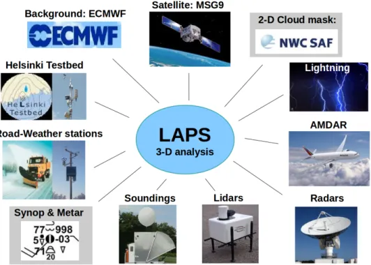
In the FMI version of LAPS (Fig. 1), hereaer FMI-LAPS (Koskinen et al., 2011), the coarser background fields are taken from the latest available forecast from the European Centre for Medium-Range Weather Forecasts (ECMWF) Integrated Forecasting System (IFS). e fine-scale structures in the resulting 3D-analysis are extracted from the observations. erefore, LAPS relies heavily on the existence of a high-resolution spatial and temporal data from observational networks and remote sensors. e horizontal grid-spacing is 3 kilometres and the domain covers all of Finland and parts of neighbouring countries. e setup uses a pressure coordinate system including 44 vertical levels, distributed with a finer resolution (e.g. 10 hPa) at lower altitudes and decreasing with height. At present, FMI-LAPS is able to process several types of in-situ and remotely sensed observations such as: radar reflectivity and radial winds, weighing gauges, road-weather observations, atmospheric soundings, SYNOPs, METARs, air-traffic observations, lidars and Meteosat-9 satellite data. ere are QC's of the input data, which are important in an automated analysis system where
Figure 1:Example of the observational datasets and background model used in LAPS at FMI.
there is a minimum of human intervention. FMI-LAPS has been especially developed to better analyse the precipitation and cloud-related fields, this in order to perform better in accumulation calculations and in wind-power estimates (as in articles I, III and II, respectively).
3.1.1. LAPS – T RB
e newly developed LAPS- Regression and Barnes (RandB) method consists of two combined precipitation-correction calculations, which are run in sequence aer each other; Regression- and Barnes methods, within the LAPS routines. e linear-regression-analysis method, used in the first step, calculates the quotient between the gauge–radar pairs from all given station-points within the LAPS area. e pairs undergo QC, based on thresholds, to prohibit dubious differences between gauge and radar values (i.e. to avoid including uncertain radar measurements and spurious surface observations). Once the QC's criteria are enforced, the remaining data form a dataset of representative gauge–radar pairs from which a linear regression
can be established, calculated with the least-square method (i.e. minimize the errors between the measurement pairs). e Regression method is used to correct the overall radar estimate at all grid-points, i.e. a constant correction over the domain for a given time-step.
In the second step, the Barnes method forces the radar field to converge towards accumulation values measured by the gauges, using an objective multi-pass telescoping strategy (Barnes, 1964; Hiemstra et al., 2006). Also here the gauge–radar quotients are used (including QC) and in order to optimize the result, several iteration steps are performed within the Barnes analysis, at successively finer scales. e corrections are weighted with distance (i.e. less impact from gauge observation further away from surface station) and rectifies the radar field in the surroundings to gauge stations.
3.1.2. LAPS – L D A (LDA)
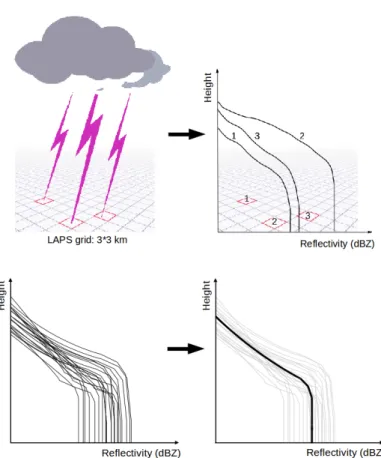
e Lightning Data Assimilation (LDA) method is constructed to build up statistical relationships between radar–lightning measurements and the new dataset is further used to improve the precipitation-accumulation estimates (article III). LDA counts the number of cloud-to-ground lightning strikes and converts lightning intensity into vertical radar-reflectivity profiles. e FMI-LAPS LDA method uses a 5 min interval of lightning and radar data, within a LAPS grid-box of resolution 3*3 km (Fig 2).
e collected strikes are divided into binned categories using an exponential division (i.e. 2n...2n+1), following the same method used in (Pessi, 2013). is results
in 6 different lightning categories (e.g. with 1, 2–3, 4–7, 8–15, 16–31 and 32–63 bins) for the Finnish lightning detection dataset. For each of these 6 categories the average reflectivity is calculated at each grid-point, for each level, and results in the final radar–lightning reflectivity profiles. For the Finland domain, the climatological radar–lightning relationship profiles were estimated using lightning information and operational radar-volume data from summer 2014. Approximately 220,000 lightning strikes were used for this calibration.
3.1.3. LAPS – LOWICE
A system to detect icing, calculating the ice load and the wind-power losses (LOWICE) has been developed by Leading Edge Atmospherics (LEA) and FMI (Gregow et al., 2015). e LOWICE model was run over the Nordic area using LAPS as its primary data source to produce gridded fields of relevant quantities for near-surface icing: temperature, humidity, winds, cloud microphysics, cloud fraction and precipitation type. LOWICE produces estimates of the following at the height of the wind turbine: wind speed, supercooled liquid water content (SLWC), drop size, icing intensity (i.e. accretion rate) and ice load.
Figure 2: Scheme of the LDA method. Lightning strikes remapped onto LAPS grid (upper-left panel), where radar-reflectivity profiles are collected for the same grid-boxes (upper-right panel). The assembled radar profiles are handled for a time-period of 5 minutes and binned into classes (lower-left panel; example of one bin) and finally, the average profile is calculated for each bin (lower-right panel; thick line).
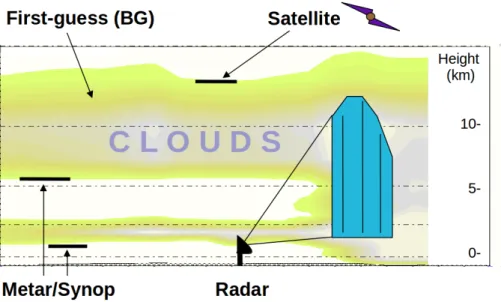
Clouds have a key role when calculating icing-related quantities, affecting wind-power turbines; and one of the main features within the FMI-developed LAPS version is the cloud-resolving process (Fig. 3). e cloud analysis is dependent on the use of satellite input, visible and infrared channels, which are used to detect the cloud-mask and estimate the cloud-top temperature/height. Additionally, information from SYNOP, METAR and radar is used to fill in the vertical cloud structure and the height of the cloud-base. New FMI-LAPS developments include the use of cloud-mask information from a NWCSAF product (Dybbroe et al., 2005) and the detection of clouds captured within temperature inversions (e.g. low clouds).
Figure 3: Sketch of how observations and NWP model are used within the FMI-LAPS cloud process. The satellite detects the cloud-top; surface stations (e.g. Metar and Synop) measures the cloud-base heights and the vertical structures of the clouds are filled together with radar measurements and first-guess fields from background (BG; from NWP forecast model).
e icing intensity is estimated using liquid water content (LWC; g m−3), the temperature and the wind speed at the height of interest (e.g 100 metres above ground level). Temperature and wind speed are interpolated from LAPS vertical levels. LOWICE estimates the LWC by calculating the change of saturation-mixing ratio between two levels, in a similar manner as (Betts, 1987). erefore, when the level of interest is located at or above the estimated cloud-base height (CBZ), the LWC is approximated by; 1) estimating the saturated-mixing ratio at CBZ, 2) taking the difference between the mixing ratios at cloud-base and the height of interest (assuming
a moist adiabatic temperature lapse rate) and finally, 3) compensating for density. Also, LOWICE is taking into account the depletion of LWC due to precipitation (especially snow), by analysing the observation reports from nearby stations. e depletion factor is depending on distance to observation and the LWC can be reduced with maximum 50% of its original value. To calculate the icing rate, with input of the atmospheric icing conditions from above, a standard icing-rate equation is used (Makkonen, 2000)
dm
dt =SLW CAvα1α2α3, (3)
whereSLW Cis the supercooled LWC,Ais the cross-sectional area of the object, v is the wind velocity; and here the collision (α1), sticking (α2) and accretion (α3)
efficiencies are set equal to 1.0. e cross-sectional area (A) is set equal to 0.015 m2, based on the ISO 12494 standard of a 0.5 m-long, 30 mm-diameter cylinder, but it could be changed to accommodate other objects (ISO, 2001). e wind speed (v; m s−1) is taken directly from LAPS. By summing the hourly icing rate and thereby
accumulating ice, when temperatures are in a suitable range, the ice load is estimated for the reference cylinder. is load will build during periods of active icing and can be depleted by melting and sublimation during periods when icing is not active. e melting scheme is currently based on temperature and the sublimation scheme use both wind speed and relative humidity.
ere are three power-loss schemes tied to the icing properties, driven by ice load and icing rate, as well as time, depending on LOWICE version. V0 uses a simple method where the build-up of ice load determines the degree of power loss (e.g. when ice load increases from 0.0 to 10.0 kg m−1, the power-loss increases linearly from 0% to 100%). LOWICE’s alternative power loss schemes (V1 and V2) combined the “building” and “clearing” effects, where ice rate and time are key factors. LOWICE versions V1 and V2 outperformed V0.
3.2. O
3.2.1. S Until the year 2013, FMI managed 77 stations instrumented with the weighing gauge Vaisala model VRG10 (used in article I). ese instruments were replaced and since 2013 FMI now operates 102 stations instrumented with the weighing gauge OTT Messtechnik Pluvio2 (used in article II). e Finnish Transport Agency (FTA) operates 370 road-weather stations with optical sensor measurements (Vaisala Present Weather Detectors models PWD11 and PWD22; used in article I and II). e FTA observation sites are not selected according to meteorological standards. Hence, their location in
the immediate vicinity of roads with heavy traffic, where “splash-effects” and wind eddies (generated by big vehicles) occasionally affect to the measurement quality and representativeness, compared to FMI stations.
3.2.2. R
As of summer 2016, FMI operated ten C-band Doppler radars where all but one of the stations have dual-polarization. At the moment, the quantitative-precipitation estimation based on dual-polarization is not used operationally but the polarimetric properties contribute to the improved clutter cancellation (i.e. removal of non-meteorological echoes; especially sea clutter, birds and insects). In FMI's general radar processing, clutter is removed with Doppler-filtering and any residual clutter with a post-processing procedure based on fuzzy logic (Peura, 2002). Additionally, the vertical profile of reflectivity (VPR) method is correcting the range-dependent errors (Zawadzki, 1984) and also compensates for overestimation in a melting layer (Koistinen et al., 2004).
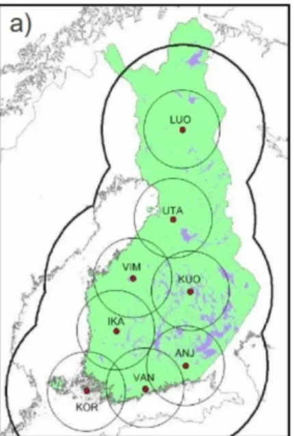
In southern Finland the distance between radars is 140–200 km, but in the north it can be as much as 260 km. e basic radar volume scan consists of thirteen PPI (so-called plan-position indicator) sweeps, which are scanned out to 250 km and repeated every 5 minutes. e location of the radars and the coverage is shown in Fig. 1a of article I. Because Finland has no high mountains, the horizon of all the radars is near zero elevation with no major beam blockage and, in general, the radar coverage is very good except in the most northern part of the country. e Finnish radar network has a very high system reliability (no interruption of data). During year 2014 and 2015 the reliability was > 99%. Further details of the FMI radar network and processing routines are described in (Saltikoff et al., 2010).
e effective radar-reflectivity factorZe(usually called reflectivity) is derived from
the expression
Ze= Per2
LC∣K∣2, (4)
wherePeis the average received microwave power,ris the measurement range,L
is the two-way attenuation in the propagation path (antenna–scatterers–antenna),Cis a radar constant (including parameters of the radar hardware) and |K| is the dielectric factor (depending on the relative fraction of ice and water in the hydrometeors).
e reflectivity uses dBZ as unit, which is expressed as
dBZ=10log10(Ze). (5)
e output of weather radars is the measured reflectivity (dBZ; Equation 4 and 5), which is further used to calculate the precipitation intensity.
3.2.3. L-
e Lightning Location System (LLS) of the FMI is part of the Nordic Lightning Information System (NORDLIS). NORDLIS started around the years 2001–2002 as a cooperation between Finland, Norway and Sweden, and gives a sufficient coverage of lightning detection for these countries. e system detects primarily cloud-to-ground strikes in the low-frequency (LF) domain, using IMPACT ES‐type sensors and a central processor; LP2000 (Cummins et al., 1998). As of 2001, another system was installed in southwest Finland, the SAFIR total lightning network with three sensors (SAFIR 3000) and a central processor. e SAFIR system is using very high frequency (VHF) interferometry to locate all lightning discharges within its coverage area and also has a separate LF, E‐field measurement for identifying ground strokes. SAFIR sensors have improved the detection efficiency and location accuracy of ground flashes in southern Finland, providing three extra time measuring stations in the network. In August 2004, a CP8000 central processor was installed which enabled the raw data from both IMPACT and SAFIR sensors to be processed at the same time. One compatible sensor (LS7000) was installed in Estonia in 2005 and was connected to FMI's central processor, which improved the detection efficiency and further widened the coverage area toward the south. At present, the FMI LLS uses this configuration: ground flash (LF) data available from Nordic countries and neighbouring areas, and cloud lightning (VHF) data that is available from SW Finland and the adjacent maritime areas.
3.2.4. I
Figure 4:Web-camera images from turbine-hub roof, on the 7th and 8th of January 2013, illustrating the visual assessment of icing. The ice-load instrument is in the centre of each image.
i.e. determined by visual inspection of web-camera images (Fig. 4). ese observations, of both the presence of ice on the instruments and its growth (active icing), are generally quite reliable. ough, in some cases they are more difficult to determine, such as when thin glazes of icing might be present or when lighting is relatively poor.
3.2.5. W-
Observations of power production were examined for several wind farms across Sweden, at locations around 800 m above sea level, over five icing seasons: 2009–2014. Because of the confidentiality agreements with wind power companies, the actual production, wind farm names, and certain other data could not be included in this thesis.
4. S
4.1. P
One main focus in the development of FMI-LAPS was to improve the precipitation accumulation estimates. e research results have been communicated to the scientific community in a series of two articles; Gregow et al. (2013) and Gregow et al. (2017).
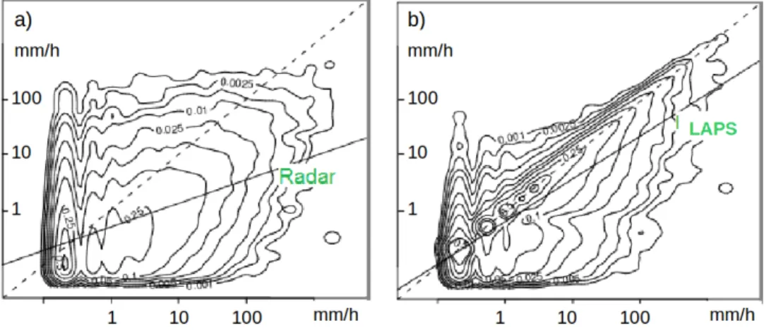
Figure 5: Verification of precipitation accumulation estimates using a) radar alone and b) LAPS-RandB method for summer 2011. Density plots of RandB analysed precipitation accumulation (y-axis: log-scale) against dependent rain-gauge observations (x-axis: log-scale). The solid line is a linear fit to the datasets and the dashed line represents the perfect 1:1 fit in the plots.
e method developed by the author (LAPS-RandB; Section 3.1.1) gives the best results when compared with already-existing methods, e.g. Regression and Barnes, and radar precipitation estimates (Fig. 5). To further investigate and verify the new RandB method, different weather situations were divided into two categories describing their airmass stability: strong convection (i.e. thunderstorms; hereaer “convective”) and light-to-moderate convection (i.e. warm-fronts; hereaer “non-convective”). Also with this categorisation, the RandB method performs best, with lower mean absolute errors (MAE) and root-mean-square errors (RMSE), compared with radar data alone (Fig. 6). Verification was done using both dependent and independent observations (i.e. observations that are or are not included, respectively, into the precipitation accumulation analysis). e performance using either the regression or Barnes assimilation analysis separately still yields better results for the accumulation products, compared to precipitation accumulation derived from radar data alone (Gregow et al., 2013).
Figure 6:Verification results for RandB method, root-mean-square errors (RMSE) and mean absolute errors (MAE), using dependent raingauge observations for two different airmass stability situations over the Finland area. Left panel: convective cases (i.e. thunderstorms) and right panel: non-convective cases (i.e. warm-fronts). The mean precipitation values, calculating the average of the raingauge data, for all the convective and non-convective cases are included as a hatched bar.
Furthermore, in a case study, the advantage of using the RandB method could be seen during a heavy-precipitation event on the 22 August 2011 at Kaisaniemi station (dependent station), located in the centre of Helsinki. For this event, the radar suffered from attenuation and gave low accumulation values (blue bar), while the LAPS-RandB method improved the analysis (red bar) and the estimated accumulation values were closer to the observed amounts (green bar; Fig. 7).
Figure 7:Case study during a heavy rainfall event, at Kaiseniemi Helsinki; 22 August 2011, 16–22 UTC. Radar-estimated precipitation accumulation (blue colour), LAPS-RandB model (red colour) and raingauge observations (green colour).
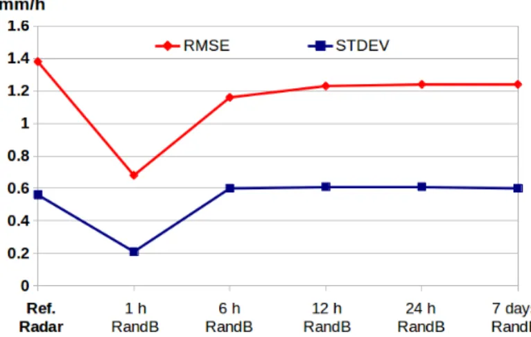
e integration time of one hour show the best result for LAPS-RandB method, when tested against a selection of longer periods (e.g. the previous 6, 12, 24 hours and 7 days of data; Fig. 8). e verification results from summer 2015 clearly indicate that the RandB method, using radar and raingauge data from the latest hour, gives the best scores for the RMSE and standard deviation (STDEV) verification values (Gregow et al., 2017).
With the use of lightning observations and the newly developed LAPS-LDA method (Section 3.1.2), heavy precipitation cases can be better resolved and the precipitation estimates improved. e studies were performed for summer periods during years 2014–2016 and the verification of the dataset also considered the distance dependencies to radar stations (i.e. gauges situated further away than 100- and 150 km), which showed the same improvement in the results. e strength of the LDA method is that the radar and lightning information can be merged and complement
Figure 8: Impact of the integration time on RandB-method for datasets during summer 2015. The scores are shown as RMSE (red colour; mm/h) and STDEV (blue; mm/h) for the different integration times, verified using independent raingauge data. The radar-estimated accumulation (Ref. Radar) scores are included as reference values.
each other. is is especially important in areas of poor, or even no, radar coverage, where the lightning information will improve the hourly precipitation accumulation analysis (Gregow et al., 2017).
4.2. W-
e LAPS-LOWICE system was developed to produce real-time, hourly estimates of the presence, intensity, and impacts of icing on wind power production. e validation results from one wind farm in January 2013 showed observed average power losses of 19.5%, while the LOWICE estimated power losses were 18.3%. Other validation results can be seen as bars in lower part of figure 9 and the graphs show that the LOWICE (versions V0, V1 and V2, respectively) compares quite well with the time-trends of turbine observed power production. It was demonstrated that wind-power energy losses due to icing were poorly correlated with ice loads. In fact, power losses were most evident when icing was active (e.g. SLWC is present and ice was actively growing at the site) and the intensity of the power losses were more strongly related to the icing rate, rather than ice load (Gregow et al., 2015).
F igur e 9: Time -ser ies for Januar y 2013 of the per cen tage of maximum po w er fr om wind tur bines (g rey), LOWICE clean po w er (blue) and ic ed po w er (r ed ,br o wn and tan lines for LOWICE versions V2, V1 and V0). C olour bars at the bott om pr o vide an hour -b y-hour assessmen t of the pr esenc e of icing as follo w s: Upper bar ;L OWICE-expec ted icing (r ed=ac tiv e icing [r at e >10g/h], yello w=inac tiv e icing [r at e <10 g/h], g reen=no icing ,whit e: no inf or ma tion). Lo w er bar ;manually assessed icing thr ough w eb -camer a (r ed=ac tiv e icing ,y ello w=ac tiv e icing possible ,but not confir med ,g reen=no ac tiv e icing ,whit e: no inf or ma tion).
5. D
LAPS is capable of using many different observations as input to its analysis and the system is being developed to use new measurements (Fig. 1). With the increase of AWS (by FMI and FTA) and the potential inclusion of data from crowdsourcing and social media (where the stations are unattended and many times the placement of a measurement is not following meteorological standards), there is a risk that data will vary in quality. Datasets may contain erroneous observations caused by for example technical problems (e.g. calibration of instruments) and physical errors (e.g. freezing of wind-anemometers or poor instrument placement), errors which might not be detected for hours or even days, depending on the provider of data. erefore, the capability to QC the observational datasets is becoming more and more important. FMI's database contains QC'ed observational datasets, data which are used within FMI-LAPS analysis. Also, FMI-LAPS is doing its own QC on several ingest parameters (outlier checks and comparison with fields from forecast model). is becomes especially important when introducing new observations (for example lightning) and with new datasets, which are not necessarily from the FMI database.
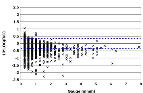
In the process of estimating precipitation accumulation, LAPS combines several different observations from raingauges, radar and lightning data. Special focus has been to improve the heavy rainfall events and weather situations which are generally characterized by relatively small spatial scales and with strong vertical motions, such as convection. ese precipitation events are known to be difficult in terms of quantitative precipitation estimation (QPE) because: (i) their small spatial scales may not be adequately sampled by gauges, and (ii) radar systems can experience problems due to attenuation of the signal, hail contamination etc. erefore, problems can occur when strong horizontal reflectivity gradients cause disagreement between radar and raingauge values, since the raingauge is a point observation while radar measures over a volume of the order of 1 km3. Vertical wind shear, along with strong winds, and hail at gauge station could also contribute to a severe mismatch between radar and gauge measurements. Despite these limitations, examples based upon disdrometer data suggest that generalized relations between two variables are useful over a wide range of remote-sensing problems and a wide range of scales (Jameson and Kostinski, 2001). Data collected over disparate sampling-volumes and sampling-frequencies can be combined to yield meaningful estimates. Although additional testing is required, this allows us to use methods which combine estimates using remote-sensing techniques with sparse but direct rainfall observations. erefore, in the FMI-LAPS radar–gauge correction method, we assume that: i) raingauge measurements are accurate for the raingauge's location, ii) radar successfully measures relative spatial and temporal variabilities of precipitation, iii) raingauge and radar measurements are valid for the same locations in time and space, and iv) relationships based on comparisons between
Figure 10:Example of the R/G quotient (y-axis in 10*log-scale) compared with raingauge observations (x-axis) from July 2015. The two blue lines indicate the 2 and 0.5 quotient, respectively.
raingauges and radars are valid for other locations in space and time (e.g. Finland and 1 hour, respectively). ough, in case the measured precipitation amount differs too much between radar and raingauge, which leads to large discrepancies in the radar–gauge quotient (as illustrated in figure 10), we limit the use of datasets. Hence, if R/G > 2 or R/G < 0.5 it is likely that the radar and raingauge do not measure the same phenomenon, at least they are uncertain values, and the raingauge data is therefore not used in field adjustment (see article I and III).
e use of the LDA represents an important source of information to improve the QPE for convective weather situations. In the LDA method, the correlation between lightning and radar is built upon statistical relationships, such as a period of approximately 1-year for the area of interest. ere are concerns regarding the spatial and timeliness representation between these two observation types. Lightning is not always collocated with the reflectivity core and the area of highest lightning frequency varies its position with respect to maximum reflectivity core over the lifetime of the storm (Lopez et al., 1990; Watson et al., 1995). Tapia et al. (1998) show that calculating the precipitation estimates using their lightning–radar method gives geographical variability and potentially exhibit substantial dependence on storm type. e variability of the spatial correlation between lightning and rainfall within the storm area suggests the use of a uniform distribution of rainfall around lightning flashes. ey
show that there is a high correlation between the temporal evolution of rainfall rate and lightning frequency, using rainfall distributed uniformly within a 10-km diameter circle around the location of the lightning strike and within 5 minutes. ese methods and results correlate with the FMI-LAPS LDA method (see article III).
Snowfall is more difficult to quantify than rain, because of the large variability in density and size of particles, which must be accounted for (Matrosov, 1998). Weather-radar systems are usually calibrated to measure the water equivalent of the reflectivity (Ze). e dielectric factor (K) included in the Ze transformation
equation is incorporated as a calibration constant, which is not altered when the precipitation form changes from liquid to solid (i.e. snow/hail/graupel). erefore, the reflectivity-rain rate (e.g. Z–R) relationship has to be changed in order to obtain a phase change of particles (Smith, 1984). Different radar-reflectivity–snow-rate relationships have been investigated throughout the years (von Lerber et al., 2017; Huang et al., 2010; Löffler-Mang and Blahak, 2001), including the use of dual-polarization radars in wintertime conditions (ompson et al., 2014). Also surface observations (i.e. raingauges) can suffer from incorrect measurements during winter-time (Martinaitis et al., 2014). erefore, the studies in this compendium focus on the liquid precipitation phase to avoid additional uncertainties of the solid phase explained above.
Satellite-precipitation products — e.g. the NWCSAF geostationary Convective Rainfall Rate (CRR) or polar orbiting Precipitating Clouds (PC) products — are planned to be included in the precipiation estimation process. e challenges with satellite based precipitation products are that the error characteristics are very different from the other measurements (Yilmaz et al., 2005) and new algorithms will need to take this into account when being developed.
Other new observations from crowdsourcing, and possibly even from social media, are becoming interesting to use within weather models. During the summer of 2017, FMI started a pilot-project to collect “citizen observations” and depending on the outcome of the project, there are opportunities to include these new datasets into for example FMI-LAPS. In the future, the variational version of LAPS is of interest because of the use of more-advanced and updated assimilation methods.
FMI-LAPS has been used as the operational analysis system since 2009 and in several other applications at the institute; calculations of gridded forecast products from Model Output Statistics; MOS (Carter et al., 1989; Glahn and Lowry, 1972) predicted station values, post-processing of radiation quantities, and hot-start of HARMONIE and other forecast models to improve the initial boundary conditions, especially hydro-meteors, and thereby improve the short-term forecast (Tiesi et al., 2016).
6. C
In order to support the FMI operational production needs, there was a clear interest to perform research with the scientific goal of improving the meteorological analysis methods underlying the identified end-user products for i) precipitation accumulation estimates and ii) icing-related quantities.
To more accurately calculate the precipitation accumulation estimate, new methods were developed within the FMI-LAPS framework. is was done by combining both the standard and new high-temporal resolution observations in new ways, taking into account the different measuring scales and error characteristics. e RandB method produces high quality gridded analysis, with improved precipitation estimates for the 1-hour integration time. Applying the LDA method lightning data does add information, especially to areas not covered by radar, and improve the results. With these developments the final precipitation accumulation product became better as of quality and temporal and spatial resolution.
e outcome of a 3-year wind-power pilot-project clearly showed the importance of high-quality meteorological fields, especially within the atmospheric boundary layer, to estimate the icing on wind-turbine blades and their effect on wind-power production. Developments of FMI-LAPS, especially cloud processes, improved the analysis of icing-related quantities (clouds, temperature, humidity etc). e newly developed icing-model LOWICE calculates wind-power production and takes into account the reduction due to icing. Using FMI-LAPS analyses as input to the newly developed icing-model, LOWICE showed good results and it was concluded that it provides useful information for the wind-power industry.
e high-quality gridded FMI-LAPS analysis products are presented at both public web-pages and within FMI in-house visualization tool (SMARTMET), and it has been found to be useful for several nowcasting purposes. Additionally, LAPS products add value when used as input to specific end-user products, such as hydrological models (used at SYKE), the FMI road-weather model and as input for the FMI fire-weather index warning delivered to the public. us far, it is clear that the use of FMI-LAPS analysis can be very useful for several applications, models, and meteorological services.
R
Albers, S. C., J. A. McGinley, D. L. Birkenheuer, and J. R. Smart, 1996: e Local Analysis and Prediction System (LAPS): Analyses of clouds, precipitation, and temperature.Weather and Forecasting,11(3), 273−287.
Barnes, S. L., 1964: A technique for maximizing details in numerical weather map analysis.Journal of Applied Meteorology,3(4), 396−409.
Barnes, S. L., 1973: Mesoscale objective map analysis using weighted time-series observations. NOAA Tech. Memo. ERL NSSL-62, National Severe Storms Laboratory, Norman, Oklahoma, 60 pp. [NTIS COM-73-10781].
Barnes, S. L., 1994: Applications of the Barnes objective analysis scheme. Part I: Effects of undersampling, wave position, and station randomness. Journal of Atmospheric and Oceanic Technology,11(6), 1433−1448.
Bauer, P., G. Ohring, C. Kummerow, and T. Auligne, 2011: Assimilating satellite observations of clouds and precipitation into NWP models.Bulletin of the American Meteorological Society,92(6), ES25−ES28.
Betts, A. K., 1987: ermodynamic constraint on the cloud liquid water feedback in climate models. Journal of Geophysical Research: Atmospheres,92(D7), 8483−8485. Carter, G. M., J. P. Dallavalle, and H. R. Glahn, 1989: Statistical forecasts based on the National Meteorological Center's numerical weather prediction system. Weather and Forecasting,4(3), 401−412.
Cattin, R., S. Kunz, A. Heimo, G. Russi, M. Russi, and M. Tiefgraber, 2007: Wind turbine ice throw studies in the Swiss Alps.European Wind Energy Conference Milan. Cummins, K. L., M. J. Murphy, E. A. Bardo, W. L. Hiscox, R. B. Pyle, and A. E. Pifer, 1998: A combined TOA/MDF technology upgrade of the US National Lightning Detection network. Journal of Geophysical Research: Atmospheres,
103(D8), 9035−9044.
Daley, R., 1991: Atmospheric data analysis, Cambridge atmospheric and space science series. Cambridge University Press,6966, 25.
Dybbroe, A., K.-G. Karlsson, and A. oss, 2005: NWCSAF AVHRR cloud detection and analysis using dynamic thresholds and radiative transfer modeling. Part I: Algorithm description.Journal of Applied Meteorology,44(1), 39−54.
Glahn, H. R., and D. A. Lowry, 1972: e use of model output statistics (MOS) in objective weather forecasting. Journal of Applied Meteorology,11(8), 1203−1211. Gregow, E., B. Bernstein, I. Wittmeyer, and J. Hirvonen, 2015: LAPS−LOWICE: A
Real-Time System for the Assessment of Low-Level Icing Conditions and eir Effect on Wind Power. Journal of Atmospheric and Oceanic Technology, 32(8), 1447−1463.
Gregow, E., A. Pessi, A. Mäkelä, and E. Saltikoff, 2017: Improving the precipitation accumulation analysis using lightning measurements and different integration periods. Hydrology and Earth System Sciences,21(1), 267.
Gregow, E., E. Saltikoff, S. Albers, and H. Hohti, 2013: Precipitation accumulation analysis−assimilation of radar-gauge measurements and validation of different methods. Hydrology and Earth System Sciences,17(10), 4109−4120.
Hāggmark, L., K.-I. Ivarsson, S. Gollvik, and P.-O. Olofsson, 2000: MESAN, an operational mesoscale analysis system. Tellus A,52(1), 2−20.
Haiden, T., A. Kann, C. Wittmann, G. Pistotnik, B. Bica, and C. Gruber, 2011: e Integrated Nowcasting through Comprehensive Analysis (INCA) system and its validation over the Eastern Alpine region.Weather and Forecasting,26(2), 166−183. Hiemstra, C. A., G. E. Liston, R. A. Pielke Sr, D. L. Birkenheuer, and S. C. Albers, 2006: Comparing Local Analysis and Prediction System (LAPS) assimilations with independent observations. Weather and forecasting,21(6), 1024−1040.
Huang, G.-J., V. Bringi, R. Cifelli, D. Hudak, and W. Petersen, 2010: A methodology to derive radar reflectivity−liquid equivalent snow rate relations using C-band radar and a 2D video disdrometer.Journal of Atmospheric and Oceanic Technology,27(4), 637−651.
Hyvärinen, O., and E. Saltikoff, 2010: Social media as a source of meteorological observations. Monthly Weather Review,138(8), 3175−3184.
ISO, E., 2001: Atmospheric icing of structures. INTERNATIONAL STANDARD. ISO,
12494.
Jameson, A., and A. Kostinski, 2001: Reconsideration of the physical and empirical origins of Z−R relations in radar meteorology. Quarterly Journal of the Royal Meteorological Society,127(572), 517−538.