Abstract—In this study, response surface models (RSMs) based on limited data are developed. Experimental cutting force data for the flat end milling process are employed to build these models. Four RSM models are developed in terms of process variables. The first model is used to build the mean cutting force. Similarly, the second, third and fourth models are used to build models for the variance, skewness and curtosis coefficients of the cutting forces. A bi-objective optimization procedure is developed and solved to generate a set of optimal process settings. An approximation scheme resulted in 6 possible objective combinations. The Pareto set of solutions (or part of) are generated for the six possible combinations. The merit of this study lies in the fact that response surfaces are built from limited data, often experienced in reality.
Index Terms—Limited Data, RSM, Multi-objective optimization, Approximations.
Nomenclature DOE Design of experiments OA Orthogonal Array
RSM Response Surface Method ANOVA Analysis of variance A, B, C Three forms of RSMs UL8 8 experiments OA, 2-levels UL27 3-Levels, 27 experiments OA
i o,β
β RSM model parameters 1
X Depth of Cut
2
X Rev/min 3
X Feed Rate 4
X Tool Diameter .
Std mean,F
F Mean Force & (Standard Deviation) 3
α Skewness of Fmean
4
α Curtosis of Fmean 4
1,...f
f First, Second.. objective function
τ Target value of Fmean
I. INTRODUCTION
Multi-disciplinary optimization (MDO) algorithms especially the dimensionality and complexity issues are addressed [16]. Variable fidelity Response Surface
Manuscript received April 16, 2009. Mohamed H. Gadallah is Associate Professor, Department of Operations Research, Institute of Statistical Studies & Research, Cairo University, Cairo, Egypt 12613 (phone: 202-37484624; fax: 202-37482533; e-mail: [email protected]).
Algorithm (RSA) are used to study the convergence using the Trust region algorithm. A comparative study is given for different sampling strategies based on Design of Experiments (DOE). Insufficient space fitting concepts in relation to response surface approximations are addressed.
The problem of capturing Pareto optimal points on non-convex frontiers with the aid of Aggregate Objective Functions (AOF) are studied [12]. Admissibility, necessary and sufficient conditions are discussed. An efficient method-using surrogate modeling to explore the design space is presented [19]. The method captures the Pareto frontier during multi-objective optimization. Issues related to convexity, cancavity and function discontinuity are discussed.
An algorithm based on the Clonal selection principle is presented [1]. Results are compared with other evolutionary algorithms. Evolutionary algorithms are claimed to be less sensitive to the shape or continuity of the Pareto Front. Quality metrics such as the two set coverage; spacing and generational distances are proposed to compare solutions. Physical Programming (PP) can foster the design intent and objectives into mathematical models [10]. The Weighted Sum (WS); The Compromise Programming (CP); and the Physical Programming (PP) are examined. The Normal Boundary method is claimed to generate Pareto Frontier in non-convex regions [3]. A similar approach was followed based on robust design optimization method [11].
The Pareto set of bi-criteria problems is a curve approximated by a hyper ellipse [9]. The approximation is achieved by means of a hyper ellipse to a minimum number of points and the hyper ellipse in explicit analytical description. The
ε
-constraint method, one criterion is optimized while the others are the additional constraints. The Tchebycheff scalarization finds the Pareto solution by minimizing a distance between the utopia and Pareto set (the utopia point is a point in the objective space obtained by optimizing each criterion independently). This method is capable of fitting only a sector of the Pareto set. The 2 methods:ε
-constraint and weighted Tchebycheff can be used to auxiliary generate Pareto solutions. The approach is circumvented when the Pareto set is adequately small [2]. An adaptive approximate model (AAM) based on polynomial Genetic Programming with partial interpolation strategy is developed [20]. The AAM is sequentially modified in such a way that the quality of fitting can be gradually enhanced. Various transformation methods are evaluated [18]. The WS approach for MOO is employed to study how well different methods in depicting the Pareto optimal sets. Convex combination of functions is desirable when generating theOptimization Formulation Based on Limited
Data and RSM: An Approximation
Pareto set. Advantages of Normalization technique are also demonstrated. Some improvements to the implicit limit state
function method are proposed [15]. The response surface is fitted by a weighted regression technique that allows fitting points weighted to their distance from true surface and estimated design point.
II. DEVELOPMENT
Interest in engineering mathematical based models is increasing. Models, once developed go through a series of refinements to describe properly the problem under study. Experimentation can alleviate the problem as it allows understanding of different phenomena involved. In this study, limited experimental data are available. The data represents a certain domain of interest. The modeler would start by developing a low order response surface model. These models are developed for the mean, standard deviation, skewness and curtosis coefficients. Analysis of variance is carried on the four models to verify sufficiency of fit. A multi-objective optimization formulation for the four objectives using a unique approximation is proposed and solved via a nonlinear constrained optimization routine developed within Matlab Environment. The four objective functions result in six bi-objective optimization problems. The designer will have several solutions corresponding to the two objectives employed one-at-a-time. Accordingly, the sequence of objectives has no effect on the resulting solution. Further, the Multi-objective problem is always a bi-objective optimization problem. This removes the issue of high number of objectives often experienced in reality. A physical process with four variables and eight experiments is studied. Both skewness and curtosis are calculated from equation 1.
Skewness Coefficient= 3
3
3 E [X ]
σ μ − =
α
Curtosis Coefficient= 4
4
4 E [X ]
σ μ − =
α
1
Where X = Fmean, μ =mean of eight force
measurements, σ=the standard deviation of the mean force.
The Fmean, Fstd, α3and α4are used to develop the models
in terms of the four variables and their interactions. Three confidence levels are used to assess adequacy of models at 99%, 95% and 90% confidence levels respectively. Table 1 gives the 8 experiments and corresponding mean and force standard deviations. Table 2 gives the significant variables using Fmean and Fstd at different confidence levels. At 90% confidence, X1,X2,X3,X2.X3,X1.X4 are significant using Fmean as a response. Similarly,
3 2 3 1 3 2
1,X ,X ,X .X ,X .X
X are significant at 90% level
using Fstd as a response. This procedure is repeated similarly at 95% and 99% confidence levels. The maximum error based on Fmean ranges from 13.76% (at 90% confidence) to 16.33% (at 99% confidence). Moreover, the maximum error based on Fstd ranges from 35.50% (at 90% confidence) to
[image:2.595.313.539.81.416.2]66.67% (at 95% confidence).
Table 1: UL8 and Mean, Fstd, Skewness and Curtosis Coefficients
Exp Input Parameters
1
X X2 X3 X4
1 1.5 800 71 8
2 1.5 800 140 12
3 1.5 1600 71 8
4 1.5 1600 140 12
5 3 800 71 12
6 3 800 140 8
7 3 1600 71 12
8 3 1600 140 8
Output Parameters
Exp
F mean F std α3 α4
1 44.47 31.60 -0.9895 0.9861
2 100.78 98.15 +0.5420 0.4419
3 32.37 20.77 -2.6616 3.6886
4 64.91 55.09 -0.0388 0.01317
5 70.56 59.45 -0.00387 0.000607
6 138.58 108.10 +8.3859 17.0368
7 67.30 65.09 -0.01796 0.004706
8 84.55 65.51 +0.02518 0.007383
Table 2: Significant variables based on different confidence levels and UL8
Confidence Level
90% 95%
Max error based on Fmean
13.76% 16.33%
Max Error based on Fstd
35.59% 66.7%
Based on Fmean
4 X . 1 X , 3 X . 2 X
, 3 X , 2 X , 1 X
3 X . 2 X
, 3 X , 2 X , 1 X
Based on Fstd
3 X . 2 X , 3 X . 1 X
, 3 X , 2 X , 1 X
3 X . 2 X
, 3 X , 2 X , 1 X
Confidence Level 99%
Max error based on Fmean 16.33%
Max Error based on Fstd -
Based on Fmean
3 X . 2 X , 3 X
, 2 X , 1 X
Based on Fstd -
[image:2.595.313.539.460.669.2]Table 3: RSM Model Coefficients for UL8 Model
Coef.
Models 0
β β1 β2 β3
A -6.1551 24.403 -0.024 0.630 B -10.657 26.227 -0.024 0.669 Fmean
C -96.155 26.2279 0.0471 1.48
A 24.076 6.9533 -0.0443 0.5433
B -35.325 33.3538 -0.0443 1.1063
Fstd.
C -127.59 33.3538 0.0326 1.9809
Model Coef.
Models 4
β β5 β6 Error
A -0.003 - - 15.80%
B -0.003 -0.0173 - 14.83%
Fmean
C -0.0039 -0.0173 -0.0007 -4.70%
A 0.0071 - - 28.52%
B 0.0071 -0.2502 - 18.66%
Fstd.
C 0.0071 -0.2502 -0.0007 13.19%
III Bi-Objective Optimization Formulation The optimization problem subject to limits on process variables is stated next as:
Minimize f1 = (Fmean−τ)
Minimize f2 = Fstd
Minimize f3 = α3
Minimize f4 = α4 Subject to: 12 4 X 8 ; 140 3 X 71 ; 1600 2 X 800 ; 0 . 3 1 X 5 . 1 ≤ ≤ ≤ ≤ ≤ ≤ ≤ ≤ Where: 3 X . 2 X 0007 . 0 3 X . 1 X 0173 . 0 2 X . 1 X 0039 . 0 3 X 48 . 1 + 2 X 0471 . 0 + 1 X 2279 . 26 + 155 . 96 = mean F 3 X . 2 X 0007 . 0 3 X . 1 X 2502 . 0 2 X . 1 X 0071 . 0 + 3 X 9809 . 1 + 2 X 0326 . 0 + 1 X 3538 . 33 + 59 . 127 = Std F 3 2 3 1 2 1 3 2 1 3 X X 0001 . 0 X X 0207 . 0 X X 0026 . 0 X 078 . 0 X 0094 . 0 X 8031 . 2 7977 . 14 − + − + + + − = α 3 2 3 1 2 1 3 2 1 4 X X 0002 . 0 X X 1027 . 0 X X 0080 . 0 X 0346 . 0 X 0328 . 0 X 8015 . 0 5231 . 21 − + − + + + − = α Approximation:
[image:3.595.311.537.145.558.2]A procedure is developed to approximate the sequence of problem approximations. The 4 objectives require 4C =6 2 approximations as given in Table 4.
Table 4: Six possible multi-objective sub-problems.
Trial ) F ( f mean 1 τ −
= f2 =Fstd f3 =α3 f4 = α4
1 9 9 - -
2 9 - 9 -
3 9 - 9
4 - 9 9 -
5 - 9 - 9
6 - - 9 9
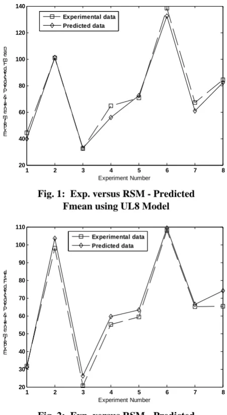
Figures 1 and 2 give the experimental vs. RSM predicted Fmean and Fstd using UL8. UL8 is an eight trial array and models the linear behavior of the experimental forces. Nonlinearities, once modeled should use three, four, five levels respectively.
1 2 3 4 5 6 7 8
20 40 60 80 100 120 140 Experiment Number Ex p eri me nta l & P re dic te d F me a n
Experimental data Predicted data
Fig. 1: Exp. versus RSM - Predicted Fmean using UL8 Model
1 2 3 4 5 6 7 8
20 30 40 50 60 70 80 90 100 110 Experiment Number Ex p eri me nta l & P re dic te d F std
Experimental data Predicted data
Fig. 2: Exp. versus RSM - Predicted Fstd. using UL8 Model
Different problems are given as: Problem # 1:
Minimize f1 = (Fmean−τ)
Minimize f2 =Fstd
Subject to: 171.5≤≤XX31≤≤1403.0;;8800≤X≤4X≤212≤1600; and 3 X 2 X 0001 . 0 3 X 1 X 0207 . 0 + 2 X 1 X 0026 . 0 3 X 078 . 0 + 2 X 0094 . 0 + 1 X 8031 . 2 + 7977 . 14 = 3 α 3 X 2 X 0002 . 0 3 X 1 X 1027 . 0 + 2 X 1 X 0080 . 0 3 X 0346 . 0 + 2 X 0328 . 0 + 1 X 8015 . 0 + 5231 . 21 = 4 α
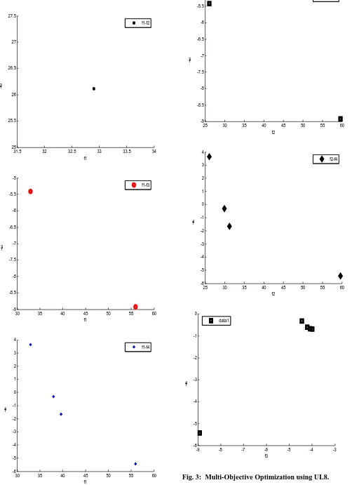
[image:3.595.48.294.674.775.2]Figure 3 gives the 6-possible approximations for the bi-objective optimization problem.
31.5 32 32.5 33 33.5 34 25
25.5 26 26.5 27 27.5
f1 f2
f1-f2
30 35 40 45 50 55 60
-9 -8.5 -8 -7.5 -7 -6.5 -6 -5.5 -5
f1 f3
f1-f3
30 35 40 45 50 55 60
-6 -5 -4 -3 -2 -1 0 1 2 3 4
f1 f4
f1-f4
25 30 35 40 45 50 55 60 -9
-8.5 -8 -7.5 -7 -6.5 -6 -5.5 -5
f2 f3
f2-f3
25 30 35 40 45 50 55 60 -6
-5 -4 -3 -2 -1 0 1 2 3 4
f2 f4
f2-f4
-9 -8 -7 -6 -5 -4 -3
-6 -5 -4 -3 -2 -1 0
f3 f4
data1
[image:4.595.55.557.82.773.2]The solutions of the multi-objective problems are shown in Appendix I. Problem 1 is a bi-objective optimization in the f1-f2 domain. X* = (1.5, 1600, 71 8) and f1*=32.9044 and f2*=26.1183. In problem 2, the f1-f3 domain, X*=(1.5, 1600, 71,8) and X*=(1.5 1600, 140, 8). The point X*=(1.5, 1600, 71, 8) repeats twice regardless of the bi-objective problem solved. A look at the optima generated by the six sub-problems, the point X*=(1.5,1600,71,8) is a common solution to all the domains. Hence, this point is certainly a point on the Pareto Frontier. The two points (1.5, 1600, 71, 8) and (1.5, 1600, 140, 8) require a bit of attention as the UL8 allows the variation of 4 variables in 2 levels. This means, 16 experiments are needed instead of 8. Since we have used only 50% of what is required, this means that X3& X4
could have been confounded. The consequence could imply that the two points may in fact be one point. Similarly, the point (1.5, 800, 71, 8) in the f1-f4 domain appears in the f2-f4 domain. The same can be stated for the point (1.5, 1000, 71,8) in the f1-f4 and f2-f4 domains respectively. The methodology developed can be depicted graphically in figure 4. Similarly, two UL27 (different domains), UL25 and UL32 are employed to develop the four equations (not shown for brevity). The resulting optima are compared and discussed versus the type and nature of array. These optima are compared via several quality indices such as: cost of solution, stability of solution, uniformity of solution, etc. Appendix II gives measurements and ANOVA for UL8. Appendix III gives the experimental vs. Predicted forces using UL27.
Start
Limited Data
Ma
th
e
m
a
tic
a
l
M
ode
l
P
roce
ss
Ex
pe
rim
e
nt
al
Se
tu
p
Analysis of Variance Based on Different Confidence Levels
90% 95% 99%
Lowest Error
Develop a RSM for Fmean, Fstd, etc.
Formulate a Multi-Objective Problem
Approximate the # of objective combinations
Solve
Assess Solutions
[image:5.595.327.529.634.758.2]End
Fig. 4: Flow Chart of Proposed Methodology
IV Conclusion
A procedure is given to develop mathematical models from limited data points. RSM is employed to optimize a set of bi-objective problems. The 2-objective functions represent the majority of optimal solutions in their planes according to the approximation given
Appendix I: Multi-objective Solutions
Objectives *
X f*=[fi*,fj*] #
2 f & 1
f (1.5, 1600, 71, 8) [32.9044, 26.1183] 1 (1.5, 1600, 71, 8) [32.9044, -5.4105] (1.5, 1600, 140, 8) [55.9538, -8.9261] 3
f & 1 f
(1.5, 1600, 71, 8) [32.9044, -5.4105] 2
(1.5, 1600, 140, 8) [55.9538, -5.4298] (1.5, 800, 71, 8) [39.6641, -1.6467] (1.5, 1000, 71, 8) [37.9744, -0.3267] 4
f & 1 f
(1.5, 1600, 71, 8) [32.9044, 3.6333] 3
(1.5, 1600, 140, 8) [52.6247, -8.9261] 3
f & 2 f
(1.5, 1600, 71, 8) [26.1183, -5.4105] 4
(1.5, 1600, 140, 8) [59.6247, -5.4298] (1.5, 800, 71, 8) [31.2783, -1.6467] (1.5, 1000, 71, 8) [29.9883, -0.3267] 4
f & 2 f
(1.5, 1600, 71, 8) [26.1183, 3.6333] 5
(1.5, 1600, 140, 8) [-8.9261, -5.4298] (1.5, 965, 103.8, 8) [-3.9837, -0.7004] (1.5, 972, 98.16, 8) [-4.0844, -0.6675] (1.5, 976, 89.04, 8) [-4.2074, -0.6017] (1.5, 1600, 71, 8) [-4.4505, -0.3267] 4
f & 3 f
(1.5, 1600, 140, 8) [-8.9261, -5.4298] 6
Appendix II: UL8OA & experimentation using either Fmean and Fstd respectively.
# 1
X X2 X1.X2 X3 X1.X3
4
X 3
2
X . X
4 1
X . X
1 1 1 1 1 1 1 1
2 1 1 1 2 2 2 2
3 1 2 2 1 1 1 2
4 1 2 2 2 2 2 1
5 2 1 2 1 2 2 2
6 2 1 2 2 1 1 1
7 2 2 1 1 2 2 1
8 2 2 1 2 1 1 2
#
mean
F FStd
1 44.47 31.60
2 100.78 98.15
3 32.37 20.77
4 64.91 55.09
5 70.56 59.45
6 138.58 108.1
7 67.30 65.09
8 84.55 65.51
T 603.52 503.76
ANOVA Results based on Fmean & Fstd using UL8.
Source SS DOF Variance Fcal
1
X 1754 1 1754 281.2
2
X 1384 1 1384 222.03
3
X 3789 1 3789 607.57
4 X . 1
X 91 1 91 14.609
3 X . 2
X 694 1 694 111.34
Error 12.475 2 6.2375
SST 7726.88 7
53 . 8 % 90 , 2 , 1
Source SS DOF Variance Fcal
1
X 1070 1 1070 31.52
2
X 1031 1 1031 30.37
3
X 2810 1 2810 82.75
) 3 X 1 X ( 4
X 335.4 1 335.4 9.877
4 X . 1
X 32 1 32 ~1
3 X 2
X 809.22 1 809.22 23.83
Error 1
SST 6124.7 7
53 . 8 % 90 , 2 , 1
F = , F1,2,95%=18.5, F1,2,99%=93.5
Appendix III: Exp vs. Predicted Fmean and Fstd using UL27OA.
0 5 10 15 20 25 30 0
50 100 150 200 250
Experiment Number Ex
peri me nta l & P re dic te d F me a n
Experimental data Predicted data
0 5 10 15 20 25 30 0
20 40 60 80 100 120 140
Experiment Number Ex
peri me nta l & P re dic te d F std .
Experimental data Predicted data
Exp vs. RSM Predicted Force Components using UL27-2 OA
ACKNOWLEDGMENT
I would like to acknowledge the valuable discussions with Professor M. Bayoumi from Cairo University.
REFERENCES
[1] Coello, C.A.C. ,Cortes, N.C., “Solving Multi-Objective Optimization Problems using an Artificial Immune System”, Kluwer Academic Publishers, 2002, pp. 1-35.
[2] Christpher, A.M., Anoop, A.M. and Messac, A., "Smart Pareto Filter: Obtaining A Minimal Representation of Multi-objective Design Space", Engineering Optimization, Vol. 36 no. 6, 2004, pp. 721-740. [3] Das, I. and J.E.Dennis, “Normal Boundary Intersection: A New Method
for Generating the Pareto Surface in Nonlinear Multi-Criteria Optimization Problems”, Department of Computational and Applied Mathematics, Rice University, Houston, TX, 1996.
[4] Fabio, F. and Mauizio, R., "VIS: An Artificial Immune Network for Multi-Objective Optimization", Engineering Optimization, Vol. 38, no.8, 2006, pp.975-996.
[5] Hongbing, Fang and Mark F. Horstemeyer, “Global Response Approximation with Radial Basis Functions”, Engineering Optimization, Vol. 38, no. 4, 2006, pp. 407-424.
[6] Jenn-Long Liu, “Novel Orthogonal Simulated Annealing with Fractional Factorial Analysis to Solve Global Optimization Problems”, Engineering Optimization, Vol. 37 no. 5, 2005, pp. 499-523. [7] Janga R. and Nagesh, K., "An Efficient Multi-Objective Optimization
Algorithm based on Swarm Intelligence foe Engineering Design", Engineering Optimization, Vol. 39, no. 1, 2007, pp. 49-68.
[8] Kok, S. Won and Tapabrata Ray, "A Framework for Design Optimization using Surrogates", Engineering Optimization, Vol. 37 no. 7, 2005, pp. 685-703.
[9] Li, Y., Fadel, G.M. Wiecek, M., Blouin, V., “Minimum Effort Approximation of the Pareto Space of Convex Bi-Criteria Problems”, J. of Optimization and Engineering, Vol. 4, 2003, pp. 231-261. [10] Messac, A. and Mattson, C. , “Generating Well Distinguished Sets of
Pareto Points frontier Engineering Design using Physical Programming”, Optimization and Engineering, Vol. 3, 2002, pp. 431-450.
[11] Messac, A., Yahia, I. , “Multi-Objective Robust Design Using Physical Programming”, Structural and Multi-Disciplinary Optimization, Vol. 23, No. 5, 2002, pp.357-371.
[12] Messac, A., Sukam, P.C., Melachrinoudis, E., “Aggregate Objective Functions and Pareto Frontiers: Required Relationships and Practical Implications”, Optimization and Engineering, Vol. 1, 2000, pp.171-188.
[13] Matlab user Manual, Version 7, The Math Works Inc., 2004.
[14] Narayanan, A., Toropov, V.V., Wood, A.S., Campean, I.F. “Simultaneous Model Building & Validation with Uniform Design of Experiments", Engineering Optimization, Vol. 39, no. 5, 2007, pp. 497-512.
[15] Nguyen X.S. Sellier, A., Duprat, F., Pons G. “Adaptive Response Surface Method based on a Double Weighted Regression Technique” Probabilistic Engineering Mechanics Vol. 24 2009, pp. 135-143. [16] Rodriguez J.F., Perez, V. M. Padmanabhan, D. and Renaud, J.E.
“Sequential Approximate Optimization using Variable Fidelty Response Surface Approximations” Structural Multi-Disciplinary Optimization Vol. 22, 2001 pp. 24-34.
[17] Shin, S., A New Paradigm for Integrated Bi-Objective Robust-Tolerance Design Modeling and Optimization, Ph.D. Dissertations, Clemson University, 2005.
[18] Timothy, R.M., Arrora, J.S., "Function Transformation Methods for Multi-Objective Optimization", Engineering Optimization, Vol. 37 no. 6, 2005, pp. 551-570.
[19] Wilson, B., Cappelleri, D., Simpson, T. Frecker, M., “Efficient Pareto Frontier Exploration using Surrogate Approximations”, Optimization and Engineering, Vol. 2, pp. 31-50, 2001.