Numerical Solution Techniques for the Steady
Incompressible Navier-Stokes Problem
M. ur Rehman
1,2C. Vuik
1,3G. Segal
1,4Abstract—In this paper we discuss some re-cently published preconditioners for the incompress-ible Navier-Stokes equations. In combination with Krylov subspace methods, they give a fast conver-gence for the solution of the Navier -Stokes equa-tions. With the help of numerical experiments, we report some new findings regarding the convergence of these preconditioners. Besides that, a renumber-ing scheme for direct solvers and ILU preconditioner is introduced that improves the convergence of the solvers. Both 2D and 3D experiments are used to measure the performance of the preconditioners. Keywords: block preconditioners, ILU preconditioners, Navier-Stokes, renumbering
1
Introduction
The incompressible Navier -Stokes equations, given as
−ν∇2u+u.∇u+∇p=f in Ω (1)
∇.u= 0 in Ω, (2) are used to simulate fluid flow in a medium with the fol-lowing properties: the fluid is incompressible and has a Newtonian character. Equation (1) represents the mo-mentum equation and (2) is the continuity equation or
mass conservation equation. ν is the viscosity (inversely
proportional to the Reynolds number), u is the
veloc-ity vector and p is the pressure. For ν → ∞ , the
sys-tem of equations in (1) and (2) tends to a linear syssys-tem of equations known as Stokes problem. The boundary value problem we consider, is system (1) and (2) posed on a two dimensional domain Ω, together with boundary
conditions on∂Ω =∂ΩD∪∂ΩN given by
u=w on ∂ΩD, ν∂u
∂n−np= 0 on ∂ΩN,
wherewis a given function.
The system given in (1) and (2) is discretized by the
1Delft University of Technology, DIAM, Mekelweg 4, 2628 CD,
Delft, The Netherlands;
email:{M.urRehman2, c.vuik3, a.segal4}@tudelft.nl Manuscript submitted for review on 22-02-2008. Reviewed manuscript submitted on 07-04-2008.
finite element method. Due to the presence of the
con-vective term (u.∇u) in the momentum equation, the
dis-cretization of the Navier -Stokes equation leads to a non-linear system of equations. The Navier -Stokes system
is linearized by Picard’s method. In the Picard
iter-ation method, the velocity from the previous iteriter-ation is substituted into the convective term. Starting with
an initial guess u(0) for the velocity field, Picard’s
it-eration constructs a sequence of approximate solutions
(u(k+1), p(k+1)) by solving a linear Oseen problem
−νΔu(k+1)+ (u(k).∇)u(k+1)+∇p(k+1)=u in Ω, (3)
∇.u(k+1)= 0 in Ω, (4)
in matrix notation
F BT
B 0
u p
=
f 0
. (5)
F=A+N, whereAis the viscous part,N is the
contri-bution of convective term linearized by Picard’s method,
BT is the gradient operator, andB is the divergence
op-erator. The linearization of the Navier -Stokes problem gives rise to a saddle point problem, which means that there is a large block of zeros at the main diagonal. Several techniques have been introduced to solve this
sys-tem efficiently. Recently various preconditioners have
been published, that can be used to accelerate the so-lution of system (5) by Krylov subspace methods [1–3]. We will discuss SIMPLE-type preconditioners as formu-lated by Vuik [3] in Section 2.
2
Preconditioners for the Navier-Stokes
Equations
Preconditioning is a technique used to enhance the con-vergence of an iterative method to solve a large linear
systems iteratively. Instead of solving a systemAx=b,
one solves a systemP−1Ax=P−1b, whereP is the
pre-conditioner. A good preconditioner should lead to fast convergence of the Krylov method. Furthermore, system
of the formP z=rshould be easy to solve.
In the Navier -Stokes equations, the objective is to de-sign a preconditioner, that increases the convergence of an iterative method independent of the Reynolds number and number of gridpoints. Secondly, the application of a preconditioner should be cheap. For more details, see [7]. We discuss here preconditioners for the incompressible Navier-Stokes equations.
2.1
SIMPLE(R) Preconditioner
SIMPLE (Semi Implicit Method for Pressure Linked Equations) [8], [9] is a classical algorithm for solving the Navier-Stokes equations, discretized by a finite volume
technique. In this algorithm, to solve the momentum
equations, the pressure is assumed to be known from the previous iteration. The newly obtained velocities do not satisfy the continuity equation since the pressure field is only a guess. Corrections to velocities and pressure are proposed to satisfy the discrete continuity equation. The
SIMPLE algorithm is derived from the blockLU
decom-position of the coefficient matrix (5)
F BT
B 0 u p = F 0
B −BF−1BT
I F−1BT
0 I u p = f g . (6)
The approximation F−1 = D−1 = diag(F)−1 in (2,2)
and (1,2) inL and U block matrices, respectively, leads
to the SIMPLE algorithm. Define
u∗ δp =
I D−1BT
0 I
u p
. (7)
First we solve
F 0
B −BD−1BT
u∗ δp = f g , (8)
and then uand p from (7). In the SIMPLE algorithm,
the above two steps are performed recursively leading to:
SIMPLE algorithm:
1. Solve F u∗=ru−BTp∗.
2. Solve ˆSδp=rp−Bu∗.
3. update u=u∗−D−1BTδp.
4. update p=p∗+δp. ,
where pressurep∗ is estimated from the prior iterations.
Dis the diagonal of the convection diffusion matrix and
ˆ
S=−BD−1BT, an approximation of the Schur
comple-ment.
Vuik et al [3], used SIMPLE and its variants as a precon-ditioner to solve the incompressible Navier-Stokes prob-lem. One iteration of the SIMPLE algorithm is used as
a preconditioner with assumptionp∗= 0. The
precondi-tioner gives nice convergence if used in combination with the GCR method. However, the convergence decreases if the number of grid elements or Reynolds number in-creases. A variant of SIMPLE, SIMPLER gives conver-gence independent of Reynolds number. Instead of
esti-mating the pressure p∗in the SIMPLE algorithm, p∗ is
obtained from solving a subsystem:
ˆ
Sp∗=rp−BD−1((D−F)uk+rv), (9)
where uk is obtained from the prior iteration. In case
SIMPLER is used as preconditioner, uk is taken equal
to zero. The classical SIMPLER algorithm proposed by Patanker consists of two pressure solves and one veloc-ity solve. However, in the literature the SIMPLER algo-rithm is formulated such that the steps of the algoalgo-rithm are closely related to the Symmetric Block Gauss-Seidal method [3]. This form of the SIMPLER preconditioner can be written as:
u∗ p∗ = uk pk
+ML−1BL
ru rp −A uk pk , (10)
uk+1
pk+1
= u∗ p∗
+BRMR−1
ru rp −A u∗ p∗ , (11)
whereArepresents the coefficient matrix given in (5),uk
andpk in (10) are obtained from the previous step (both
zero in our case) and
BR=
I −D−1BT
0 I
, MR=
F 0
B Sˆ
and (12)
BL=
I 0
−BD−1 I
, ML=
F BT
0 Sˆ
. (13)
3
Reordering Scheme for LU/ILU
Fac-torization
In this section we will discuss an a priori renumbering scheme to use both in the ILU preconditioner and a direct solver to solve the Navier-Stokes problem. From a practi-cal point of view, it would be attractive, if standard classi-cal iterative solution schemes, like preconditioned Krylov solvers, could be applied, without any changes. However, in the case of non-stabilized elements, the zero pressure block in the continuity equation, prevents straightforward application of LU and ILU factorization. If the common ordering of unknowns is used, i.e. placing first all un-knowns of node 1, then those of node 2 and so on, one might get a zero pivot, especially if velocities at some boundaries are prescribed and therefore both factoriza-tions may fail. Pivoting, on the other hand, will result in a large increase of memory usage and, as a consequence, computation time. Besides that, it is hard, to predict, a priori, the amount of memory required, which from an implementation point of view is, not very practical. To avoid this problem, it is better to use a suitable a priori reordering of unknowns. We propose a new ordering that avoids breakdown of LU factorization. Our reordering schemes consist of two steps.
1. Renumbering of grid points, that can be accom-plished by any renumbering method that gives an optimal profile. We use Cuthill McKee (CMK) [10] and Sloan [11] renumbering schemes for grid points.
2. The second step consisits of reordering of unknowns. Unknowns can be reordered as first all the veloc-ity unknowns, followed by pressure unknowns in the
grid. This is know as p-last ordering.
A new type of reordering is introduced, in which the grid is divided into levels. Each level consists of a connected set of nodes. Thereafter, the unknowns are ordered per level. At each level, first velocity unknowns are placed and then followed by the
pres-sure unknowns. We call itp-last per level reordering.
Let us define the notion of levels for Cuthill McKee.
Sup-pose we have created levels 1 toi-1. Then leveli is
de-fined as the set of nodes that are connected directly to
leveli-1, and are not in one of the prior levels. Nodes are
connected if they belong to the same element.
The first level may be defined as a point, or even a line in
R2 or a surface inR3. In the p-last per level reordering,
one has to be careful at the start of this process. If, for example, the velocities in the first node, are prescribed, we start with a pressure unknown that gives rise to a zero pivot. Therefore, we always combine the first few levels, into a new level. If the number of free velocity unknowns in this new level, is less than the number of pressure un-knowns, we also add the next level to level 1, and if nec-essary this process is repeated. In practice combinations
of 2 or 3 levels is sufficient. Note that the starting level has always a small contribution to the global profile [12].
3.1
Direct Solver
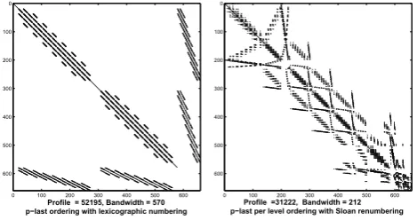
If, for a direct solver, we use the p-last ordering, we end up with a very large profile of the matrix. This is true even if we use an optimal node renumbering. The main advantage of ordering is that no pivoting is necessary, since during factorization, the zeros on the main diagonal in the zero pressure block disappear, see for example [5]. On the other hand, p-last per level, in combination with a suitable node renumbering strategy, produces a nearly optimal profile shown in Figure (1) and avoids the need for pivoting in case of direct solvers. It has been applied to many practical problems, without ever producing small pivots.
0 100 200 300 400 500 600
0
100
200
300
400
500
600
Profile = 52195, Bandwidth = 570 p−last ordering with lexicographic numbering
0 100 200 300 400 500 600
0
100
200
300
400
500
600
[image:3.595.295.530.273.397.2]Profile =31222, Bandwidth = 212 p−last per level ordering with Sloan renumbering
Figure 1: Effect of Sloan renumbering of grid points and p-last per level reordering of unknowns on the profile and bandwidth of the matrix
3.2
ILU Preconditioner
Since an optimal ordering of unknowns for a direct solver, usually improves the behavior of an ILU preconditioner, we investigate p-last per level ordering, as well as p-last ordering, in combination with ILU. The sparseness structure is defined as follows:
(LD−1U)i,j= 0 for (i, j)∈ S,
(14)
We define the set,S, of fill-in positions as the set of
un-knowns, that are directly connected. This implies that,
zeros in the pressure block, are also part of the setS,
pro-vided that there is a connectivity with velocity unknowns. In our experiments, p-last per level in combination with a suitable renumbering for grid points is used. We have
observed that p-last per level improves the convergence
3.3
Breakdown of LU or ILU Factorization
Our strategy of p-last per level does not break down. The breakdown of the ILU and LU due to p-last per level is only based on the choice of the first level. In many cases the first level contains prescribed boundary points. It might happen that our selected level gives rise to the pressure as a first row in the matrix, that in turn gives rise to a zero on the main diagonal. Therefore we kept our first level larger than the other levels. The question is, what should be the minimum number of points or nodes(unprescribed) in the first level so that our scheme encounter a danger of breakdown?
To explain how the minimum size of the first level must
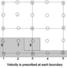
be chosen we consider a 2×2 Q2-Q1, Taylor-Hood
ele-ment subdivision of a square shown in Figure (2). If all the velocities at the boundary are prescribed, restricting the initial set to the (oblique) dashed region, i.e. nodes 1 to 7, implies that in set 1 we have only 2 unknown ve-locities and 4 unknown pressures. Even if we start with the velocities, Gaussian elimination in these rows will not remove all zeros on the diagonal. This is the same reason why we have to satisfy the LBB condition. Adding node 8 to the dashed region makes the number of velocity un-knowns in the first level equal to the number of pressure unknowns and the problem no longer exists.
[image:4.595.108.217.429.540.2]So on the first level we need at least the same number of unprescribed velocity degrees of freedom as there are pressure degree of freedom. Furthermore, the velocity un-knowns should have a nonzero connection with the pres-sure unknowns.
Figure 2: 2x2 Q2-Q1 grid
4
Numerical Experiments
Numerical experiments are performed for the following benchmark problems:
1. Driven cavity problem; flow in a square cavity with enclosed boundary conditions and a lid moving from left to right given as:
y= 1; −1≤x≤1|ux= 1−x4,
known as regularized cavity problem.
2. The L-shaped domain (−1, L)×(−1,1), known as
the backward facing step. A Poisseuille flow profile is
imposed on the inflow (x=−1; 0≤y≤1) and zero
velocity conditions are imposed on the walls. Neu-mann conditions are applied at the outflow which au-tomatically sets the mean outflow pressure to zero. Results are also performed in a 3D backward facing step.
The GCR method, [13] PCG [14], and Bi-CGSTAB [15]
are used in our experiments. Both direct solvers and
ILU preconditioners are used to solve subsystems in
the SIMPLE-type preconditioners. We divide the
experiments into two sections; Section 4.1 which deals only with SIMPLE-type preconditioners and Section 4.2 which consists of a comparison of SIMPLE-type precon-ditioners with our ILU preconditioner. The iteration is
stopped if the linear systems satisfy rk2
b2 ≤ tol, where
rk is the residual at thekthstep of the Krylov subspace
method, b is the right hand side, andtol is the desired
tolerance value. Some abbreviations used are: It.(s) are
used for number of iterations (time in seconds) and NC for no convergence and the accuracy of the inner solvers in the SIMPLER preconditioner is represented in the
form 10p,u,p (exponent for the pressure solve, velocity
solve and pressure solve), while in SIMPLE, pressure is
computed with accuracy 10−2 and the velocity 10−1 in
the preconditioning steps. The grid size in the tables and figures refer to the number of Q2-Q1 elements. Numerical experiments are performed on the system
Intel 2.66 GHz processor with 8GB RAM.
4.1
SIMPLE-type Preconditioners
ac-curacies will have no large effect on the convergence of the SIMPLE preconditioner.
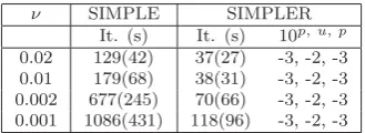
The Navier-Stokes problem solved with varying Reynolds numbers is shown in Table (2) . We report here the num-ber of iterations taken by preconditioned solver after one Picard step. We see that SIMPLER is converging faster than SIMPLE. However, SIMPLER requires some suit-able inner accuracy for convergence. From the tsuit-able, it is clear that the inner accuracy problem arises only due to the increase in the number of grid elements. As the viscosity decreases, the number of iterations of the both preconditioners increases. This increase is large in the SIMPLE preconditioner and mild in SIMPLER. Viscos-ity independent convergence with the SIMPLER precon-ditioner can be achieved only if subsystems are solved with a high accuracy.
Grid SIMPLE SIMPLER
[image:5.595.39.295.250.319.2]- Exact Inexact Exact Inexact accuracy It. (s) It. (s) It. (s) It. (s) 10p, u, p 8×8 20(0.13) 25(0.19) 10(0.07) 14(0.14) -2, -1, -2 16×16 37(1.84) 45(1.75) 15(0.89) 19(0.2) -2, -1, -3 32×32 71(14.5) 89(24.8) 24(5.3) 40(12.6) -2, -1, -3 64×64 121(132) 165(362) 40(47.5) 49(183) -3, -2, -4
Table 1: Solution of the Stokes cavity flow problem with
preconditioned GCR(20) method with accuracy 10−6
ν SIMPLE SIMPLER
[image:5.595.78.243.386.446.2]It. (s) It. (s) 10p, u, p 0.02 129(42) 37(27) -3, -2, -3 0.01 179(68) 38(31) -3, -2, -3 0.002 677(245) 70(66) -3, -2, -3 0.001 1086(431) 118(96) -3, -2, -3
Table 2: The Navier-Stokes cavity flow problem with
pre-conditioned GCR(20) method with accuracy 10−6,
sub-system in the preconditioners are solved inexactly with ILU preconditioned Bi-CGSTAB.
4.2
Comparison:
ILU Preconditioner and
SIMPLE-type Preconditioner
In this section, we report our findings with our renum-bering scheme. Our renumrenum-bering scheme effectively re-duces the profile and bandwidth of the matrix. In Table 3, we see the reduction with Sloan and Cuthill McKee renumbering method with p-last per level reordering of unknowns. Profile and bandwidth reduction is computed by dividing profile and bandwith with p-last by p-last per level. Profile reduction with the Sloan method is bet-ter than Cuthill McKee, while in bandwidth reduction Cuthill McKee performs better than Sloan. Thus, our reordering method reduces the memory and work and computation time if system is solved with a direct solver. The renumbering of grid points and reordering of un-knowns is used in the ILU preconditioner to solve the
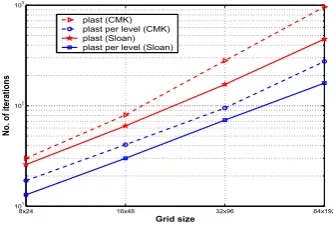
Stokes and Navier-Stokes problem. In Figure (3), we see that
• in p-last per level with Sloan and CMK give
conver-gence faster than p-last for 2D backward facing step Stokes problem,
• p-last per level with Sloan renumbering is faster than
p-last per level with CMK renumbering,
• the number of iterations increases with the increase
in the number of grid elements.
In the onward experiments, p-last per level reordering of unknowns will be used in combination with the Sloan and CMK renumbering schemes.
The 3D Stokes and the Navier-Stokes backward facing step problem is solved with the preconditioners discussed
in this paper. Results given in Table (4) and (5)
re-veal that our renumbering method performs better than the block preconditioners. In 2D the ILU preconditioner with the Sloan renumbering is performing faster than ILU computed with CMK, however in 3D, this is the other way around. ILU with CMK renumbering gives better con-vergence than the Sloan renumbering. The SIMPLER preconditioner seems to be not applicable without accu-rate inner solvers which makes SIMPLER an expensive option to use as preconditioner. For the last two problems in Table (4) and (5), convergence is achieved with the
ac-curacy higher than 10−4for the subsystem solves in the
SIMPLER preconditioner. On the other hand SIMPLE shows robust convergence behavior with approximate in-ner solves. A common aspect of all these preconditioin-ners is that convergence with these preconditioner is depen-dent on grid size.
Grid Profile reduction Bandwidth reduction
- Sloan CMK Sloan CMK
4×12 0.37 0.61 0.18 0.17
8×24 0.28 0.54 0.13 0.08
16×48 0.26 0.5 0.11 0.04
32×96 0.25 0.48 0.06 0.02
Table 3: Profile and bandwidth reduction in the back-ward facing step with Q2-Q1 discretization
Grid SIMPLE SIMPLER CMK Sloan
It.(s) It.(s) It.(s) It.(s) 8×8×24 44(6.4) 30(6) 43(1.1) 65(1.54) 16×16×48 75(155) 60(460) 118(28) 228(54) 24×24×72 108(892) NC 224(197) 479(414)
Table 4: Solution of the 3D Stokes backward facing step
[image:5.595.316.521.495.556.2] [image:5.595.295.539.624.675.2]8x24 16x48 32x96 64x192
101
102
103
Grid size
No. of iterations
plast (CMK) plast per level (CMK) plast (Sloan) plast per level (Sloan)
Figure 3: The 2D Stokes backward facing step prob-lem solved with ILU preconditioned Bi-CGSTAB method
with accuracy 10−6.
ν SIMPLE SIMPLER CMK Sloan Picard
It.(s) It.(s) It.(s) It.(s) It.
[image:6.595.77.244.48.161.2]0.02 300(789) 92(869) 225(120) 271(159) 7 0.01 464(1150) 115(925) 311(159) 368(200) 9 0.004 773(1448) 155(919) 856(317) 649(293) 12
Table 5: Solution of the 3D Navier-Stokes backward
fac-ing step (16×16×48) with preconditioned GCR(20) with
accuracy 10−2and 10−4 in the Picard linearization. The
accumulated number of iterations are reported here.
5
Conclusions
In this paper, various preconditioners for the discretized Navier-Stokes equations have been compared. A SIM-PLE -type and ILU preconditioner with special renum-bering scheme is discussed in this paper.
In the SIMPLE-type preconditioner, in 2D experiments it is observed that SIMPLER performs better than SIM-PLE. However convergence with the SIMPLER precon-ditioner strongly depends on accuracies of the subsystem solvers. Increase in the problem size, hardens the de-mand to use accurate inner solver. This limits the use of the SIMPLER preconditioner in 3D. On the other hand, though SIMPLE converges in more outer iterations than SIMPLER, it does not require an increase of the accu-racy of the inner subsystem. This makes the SIMPLE preconditioner usable for a wide range of problems. The viscosity independent convergence of SIMPLER can only be achieved with exact solves for the subsystem in the preconditioner.
In our ILU preconditioner, p-last per level reordering scheme gives better convergence than p-last . p-last per level reordering reduces the profile and bandwith of the matrix and avoids breakdown of LU/ILU. In 2D, with p-last per level reordering, Sloan performs better than CMK. In 3D, CMK gives faster convergence than Sloan. The convergence of all these preconditioners strongly de-pends on the grid size. Compared to the other precondi-tioner discussed, SIMPLE convergence is more effected by the decrease in the viscosity. Besides simple and cheaper implementation, our ILU preconditioner performs better
than SIMPLE-type preconditioners.
References
[1] M. Benzi and M. A. Olshanskii. An Augmented Lagrangian-Based Approach to the Oseen Problem.
SIAM J. Sci. Comput., 28(6):2095–2113, 2006.
[2] H. Elman, V. E. Howle, J. Shadid, R . Shuttleworth, and R. Tuminaro. Block Preconditioners Based on Approxi-mate Commutators. SIAM J. Sci. Comput., 27(5):1651– 1668, 2006.
[3] C. Vuik, A. Saghir, and G. P. Boerstoel. The Krylov ac-celerated SIMPLE(R) method for flow problems in indus-trial furnaces. Int. J. Numer. Meth. Fluids, 33(7):1027– 1040, 2000.
[4] O. Dahl and S. Ø. Wille. An ILU preconditioner with coupled node fill-in for iterative solution of the mixed fi-nite element formulation of the 2D and 3D Navier-Stokes equations. Int. J. Numer. Meth. Fluids, 15(5):525–544, 1992.
[5] S. Ø. Wille and A. F. D. Loula. A priori pivoting in solving the Navier-Stokes equations. Commun. Numer. Meth. Engng., 18(10):691–698, 2002.
[6] S. Ø. Wille, O. Staff, and A. F. D. Loula. Efficient a priori pivoting schemes for a sparse direct Gaussian equation solver for the mixed finite element formulation of the Navier-Stokes equations. Appl. Math. Modelling, 28(7):607–616, July 2004.
[7] M. Benzi, G. H. Golub, and J. Liesen. Numerical solution of saddle point problems.Acta Numerica, 14:1–137, 2005.
[8] P. Wesseling.Principles of computational fluid dynamics, volume 29. Springer Series in Computational Mathemat-ics, Springer, Heidelberg, 2001.
[9] S. V. Patankar. Numerical heat transfer and fluid flow. McGraw-Hill, New York, 1980.
[10] E. Cuthill and J. McKee. Reducing the bandwidth of sparse symmetric matrices. In Proceedings of the 1969 24th national conference, pages 157–172. ACM Press, 1969.
[11] S. W. Sloan. An algorithm for profile and wavefront re-duction of sparse matrices.Int. J. Numer. Meth. Engng., 23(2):239–251, 1986.
[12] M. ur Rehman, C. Vuik, and G. Segal. A comparison of preconditioners for incompressible Navier-Stokes solvers.
International Journal for Numerical Methods in Fluids, Electronic print available (Early view), 2007.
[13] C. Eisenstat, H. C. Elman, , and M. H. Schultz. Vari-ational iterative methods for nonsymmetric systems of linear equations. SIAM J. Numer. Anal., 20(2):345–357, April 1983.
[14] M. R. Hestenes and E. Stiefel. Methods of conjugate gradients for solving linear systems.Journal of Research of the National Bureau of Standards, 49:409–435, 1952.
[image:6.595.39.294.222.273.2]