A Graph based Approach for Contextual Text Normalization

A Graph-based Approach for Contextual Text Normalization

C¸a˘gıl S¨onmez and Arzucan ¨Ozg¨ur

Department of Computer Engineering Bogazici University

Bebek, 34342 Istanbul, Turkey

{cagil.ulusahin,arzucan.ozgur}@boun.edu.tr

Abstract

The informal nature of social media text renders it very difficult to be automati-cally processed by natural language pro-cessing tools. Text normalization, which corresponds to restoring the non-standard words to their canonical forms, provides a solution to this challenge. We introduce an unsupervised text normalization approach that utilizes not only lexical, but also con-textual and grammatical features of social text. The contextual and grammatical fea-tures are extracted from a word association graph built by using a large unlabeled so-cial media text corpus. The graph encodes the relative positions of the words with re-spect to each other, as well as their part-of-speech tags. The lexical features are ob-tained by using the longest common sub-sequence ratio and edit distance measures to encode the surface similarity among words, and the double metaphone algo-rithm to represent the phonetic similarity. Unlike most of the recent approaches that are based on generating normalization dic-tionaries, the proposed approach performs normalization by considering the context of the non-standard words in the input text. Our results show that it achieves state-of-the-art F-score performance on standard datasets. In addition, the system can be tuned to achieve very high precision with-out sacrificing much from recall.

1 Introduction

Social text, which has been growing and evolving steadily, has its own lexical and grammatical fea-tures (Choudhury et al., 2007; Eisenstein, 2013).

lolmeaninglaughing out loud,xoxomeaning kiss-ing,4umeaningfor youare among the most com-monly used examples of this jargon. In addition, these informal expressions in social text usually take many different lexical forms when generated by different individuals (Eisenstein, 2013). The limited accuracies of the Speech-to-Text (STT) tools in mobile devices, which are increasingly be-ing used to post messages on social media plat-forms, along with the scarcity of attention of the users result in additional divergence of so-cial text from more standard text such as from the newswire domain. Tools such as spellchecker and slang dictionaries have been shown to be in-sufficient to cope with this challenge long time ago (Sproat et al., 2001). In addition, most Nat-ural Language Processing (NLP) tools including named entity recognizers and dependency parsers generally perform poorly on social text (Ritter et al., 2010).

Text normalization is a preprocessing step to restore non-standard words in text to their origi-nal (canonical) forms to make use in NLP applica-tions or more broadly to understand the digitized text better (Han and Baldwin, 2011). For exam-ple,talk 2 u latercan be normalized astalk to you lateror similarlyenormoooos, enrmssand enour-moscan be normalized asenormous. Other exam-ples of text messages from Twitter and their corre-sponding normalized forms are shown in Table 1.

The non-standard words in text are referred to as Out of Vocabulary (OOV) words. The nor-malization task restores the OOV words to their In Vocabulary (IV) forms. Social text is contin-uously evolving with new words and named en-tities that are not in the vocabularies of the sys-tems (Hassan and Menezes, 2013). Therefore, not every OOV word (e.g. iPhone, WikiLeaks or

Hav guts to say wat u desire.. Dnt beat behind da bush!!

And 1 mre thng no mre sayyr people’s man!! Have guts to say what you desire.. Don’t beat behind the bush!!And one more thing no more sayyouare people’s man!! There r sm songs u don’t want 2 listen 2 yl walking cos

when u start dancing ppl won’t knwy. There are some songs you don’t want to listen to while walkingbecause when you start dancing people won’t knowwhy. Table 1: Sample tweets and their normalized forms.

enizing) should be considered for normalization. The OOV tokens that should be considered for normalization are referred to as ill-formed words. Ill-formed words can be normalized to different canonical words depending on the context of the text. For example, let’s consider the two examples in Table 1. “y” is normalized as “you” in the first one and as “why” in the second one.

In this paper, we propose a graph-based text normalization method that utilizes both contex-tual and grammatical features of social text. The contextual information of words is modeled by a word association graph that is created from a large social media text corpus. The graph repre-sents the relative positions of the words in the so-cial media text messages and their Part-of-Speech (POS) tags. The lexical similarity features among the words are modeled using the longest common subsequence ratio and edit distance that encode the surface similarity and the double metaphone algorithm that encodes the phonetic similarity. The proposed approach is unsupervised, which is an important advantage over supervised systems, given the continuously evolving language in the social media domain. The same OOV word may have different appropriate normalizations depend-ing on the context of the input text message. Re-cently proposed dictionary-based text normaliza-tion systems perform dicnormaliza-tionary look-up and al-ways normalize the same OOV word to the same IV word regardless of the context of the input text (Han et al., 2012; Hassan and Menezes, 2013). On the other hand, the proposed approach does not only make use of the general context information in a large corpus of social media text, but it also makes use of the context of the OOV word in the input text message. Thus, an OOV word can be normalized to different IV words depending on the context of the input text.

2 Related Work

Early work on text normalization mostly made use of the noisy channel model. The first work that had a significant performance improvement over the previous research was by Brill and Moore

(2000). They proposed a novel noisy channel model for spell checking based on string to string edits. Their model depended on probabilistic mod-eling of sub-string transformations.

Toutanova and Moore (2002) improved this ap-proach by extending the error model with phonetic similarities over words. Their approach is based on learning rules to predict the pronunciation of a single letter in the word depending on the neigh-bouring letters in the word.

Choudhury et al. (2007) developed a super-vised Hidden Markov Model based approach for normalizing Short Message Service (SMS) texts. They proposed a word for word decoding ap-proach and used a dictionary based method to normalize commonly used abbreviations and non-standard usage (e.g. “howz” to “how are” or “aint” to “are not”). Cook and Stevenson (2009) extended this model by introducing an unsuper-vised noisy channel model. Rather than using one generic model for all word formations as in (Choudhury et al., 2007), they used a mix-ture model in which each different word formation type is modeled explicitly.

The limitations of these methods were that they did not consider contextual features and assumed that tokens have unique normalizations. In the text normalization task several OOV tokens are am-biguous and without contextual information it is not possible to build models that can disambiguate transformations correctly.

Aw et al. (2006) proposed a phrase-based statis-tical machine translation (MT) model for the text normalization task. They defined the problem as translating the SMS language to the English lan-guage and based their model on two submodels: a word based language model and a phrase based lexical mapping model (channel model). Their system also benefits from the input context and they argue that the strength of their model is in its ability to disambiguate mapping as in “2” →

Pennell and Liu (2011) on the other hand, pro-posed a character level MT system, that is robust to new abbreviations. In their two phased system, a character level trained MT model is used to pro-duce word hypotheses and a trigram LM is used to choose a hypothesis that fits into the input context. The MT based models are supervised models, a drawback of which is that they require anno-tated data. Annoanno-tated training data is not readily available and is difficult to create especially for the rapidly evolving social media text (Yang and Eisenstein, 2013).

More recent approaches handled the text nor-malization task by building nornor-malization lexi-cons. Han and Baldwin (2011) developed a two phased model, where they only consider the ill-formed OOV words for normalization. First, a confusion set is generated using the lexical and phonetic distance features. Later, the candidates in the confusion set are ranked using a mixture of dictionary look up, word similarity based on lexical edit distance, phonemic edit distance, pre-fix sub-string, sufpre-fix sub-string and longest com-mon subsequence (LCS), as well as context sup-port metrics. Chrupala (2014) on the other hand achieved lower word error rates without using any lexical resources.

Gouws et al. (2011) investigated the distinct contributions of features that are highly depended on user-centric information such as the geologi-cal location of the users and the twitter client that the tweet is received from. Using such user-based contextual metrics they modelled the transforma-tion distributransforma-tions across populatransforma-tions.

Liu et al. (2012) proposed a broad coverage nor-malization system, which integrates an extended noisy channel model, that is based on enhanced letter transformations, visual priming, string and phonetic similarity. They try to improve the per-formance of the topnnormalization candidates by integrating human perspective modeling.

Yang and Eisenstein (2013) introduced an unsu-pervised log linear model for text normalization. Their joint statistical approach uses local context based on language modeling and surface similar-ity. Along with dictionary based models, Yang and Eisenstein’s model have obtained a significant im-provement on the performance of text normaliza-tion systems.

Another relevant study is conducted by Hassan and Menezes (2013), who generated a

normaliza-tion lexicon using Markov random walks on a con-textual similarity lattice that they created using 5-gram sequences of words. The best normaliza-tion candidates are chosen using the average hit-ting time and lexical similarity features. Context of a word in the center of a 5-gram sequence is de-fined by the other words in the 5-gram. Even if one word is not the same, the context is considered to be different. This is a relatively conservative way for modeling the prior contexts of words. In our model, we filtered candidate words based on their grammatical properties and let each neighbouring token to contribute to the prior context of a word, which leads to both a higher recall and a higher precision.

3 Methodology

In this paper, we propose a graph-based approach that models both contextual and lexical similar-ity features among an ill-formed OOV word and candidate IV words. An input text is first prepro-cessed by tokenizing and Part-Of-Speech (POS) tagging. If the text contains an OOV word, the normalization candidates are chosen by making use of the contextual features, which are extracted from a pre-generated directed word association graph, as well as lexical similarity features. Lexi-cal similarity features are based on edit distance, longest common subsequence ratio, and double metaphone distance. In addition, a slang dictio-nary1 _{is used as an external resource to enrich}

the normalization candidate set. The details of the approach are explained in the following sub-sections.

3.1 Preprocessing

After tokenization, the next step in the pipeline is POS tagging each token using a POS tagger specifically designed for social media text. Unlike the regular POS taggers designed for well-written newswire-like text, social media POS taggers pro-vide a broader set of tags specific to the peculiari-ties of social text (Owoputi et al., 2013; Gimpel et al., 2011). Using this extended set of tags we can identify tokens such as discourse markers (e.g. rt for retweets, cont. for a tweet whose content fol-lows up in the coming tweet) or URLs. This en-ables us to model better the context of the words in social media text. A sample preprocessed sentence is shown in Table 3.

As shown in Table 2, after preprocessing, each token is assigned a POS tag with a confidence score between 0 and 12_{. Later, we use these}

confi-dence scores in calculating the edge weights in our context graph. Note that even though the wordsw

and beatiful are misspelled, they are tagged cor-rectly by the tagger, with lower confidence scores though.

Token POS tag Tag confidence with Preposition 0.9963

a Determiner 0.9980

beautiful Adjective 0.9971

smile Noun 0.9712

w Preposition 0.7486

a Determiner 0.9920

beatiful Adjective 0.9733

smile Noun 0.9806

Table 2: Sample POS tagger output

3.2 Graph construction

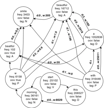
Contextual information of words is modeled through a word association graph created by us-ing a large corpus of social media text. The graph encodes the relative positions of the POS tagged words in the text with respect to each other. Af-ter preprocessing, each text message in the corpus is traversed in order to extract the nodes and the edges of the graph. A node is defined with four properties:id, oov, freqandtag. The token itself is theidfield. Thefreqproperty indicates the node’s frequency count in the dataset. Theoovfield is set to True if the token is an OOV word. Following the prior work by Han and Baldwin, (2011) we used the GNU Aspell dictionary (v0.60.6) to determine whether a word is OOV or not. We also edited the output of Aspell dictionary to accept letters other than “a” and “i” as OOV words. A portion of the graph that covers parts of the sample sentence in Table 3 is shown in Figure 1.

In the created word association graph, each node is a unique set of a token and its POS tag. This helps us to identify the candidate IV words for a given OOV word by considering not only lexical and contextual similarity, but also gram-matical similarity in terms of POS tags. For ex-ample, if the tokensmilehas been frequently seen as a Noun or a Verb, and not in other forms in the dataset (e.g. Table 4), this provides evidence that it is not a good normalization candidate for an OOV token that has been tagged as a Pronoun. On the

2_{CMU Ark Tagger (v0.3.2)}

Figure 1: Portion of the word association graph for part of the sample sentence in Table 3. (d: dis-tance, w: edge weight).

other hand, smile can be a good candidate for a Noun or a Verb OOV token, if it is lexically and contextually similar to it.

node id freq oov tag

smile 3 False A

smile 3403 False N smile 2796 False V

Table 4: The different nodes in the word associ-ation graph representing the token smile tagged with different POS tags.

An edge is created between two nodes in the graph, if the corresponding word pair (i.e. to-ken/POS pair) are contextually associated. Two words are considered to be contextually associated if they satisfy the following criteria:

• The two words co-occur within a maximum word distance of tdistance in a text message

in the corpus.

• Each word has a minimum frequency of tfrequencyin the corpus.

Let’sL startV thisD morningN wP aD beatifulA smileN .C

Table 3: Sample tokenized, POS tagged sentence (L: nominal+verbal, V: verb, D: determiner, N: noun, P: Preposition, A: adjective, C: punctuation).

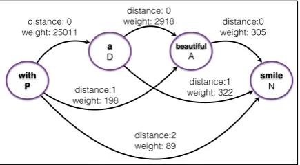
from a text including the phrase “with a beautiful smile”. The direction (from,to) and the distance together represent a unique triplet. For each pair of nodes with a specific distance there is an edge with a positive weight, if the two nodes are con-textually associated. Each co-occurrence of two contextually associated nodes increases the weight of the edge between them with an average of the nodes’ POS tag confidence scores in the text mes-sage considered. If we are to expand the graph with the example phrase “with a beautiful smile”, the weight of the edge with distance 2 from the nodewith|Pto the nodesmile|Nwould increase by

(0.9963 + 0.9712)/2, since the confidence score of the POS tag for the tokenwithis0.9963and the confidence score of the POS tag of the tokensmile

is0.9712as shown in Table 2.

20

with!

P

a! D

smile! N distance: 0

weight: 25011

beautiful!

A distance: 0

weight: 2918 distance:0 weight: 305

distance:1 weight: 322 distance:1

weight: 198

distance:2 weight: 89

Figure 2: Sample nodes and edges from the word association graph.

3.3 Graph-based Contextual Similarity Our graph-based contextual similarity method is based on the assumption that an IV word that is the canonical form of an OOV word appears in the same context with the corresponding OOV word. In other words, the two nodes in the graph share several neighbors that co-occur within the same distances to the corresponding two words in social media text. We also assume that an OOV word and its canonical form should have the same POS tag.

Given an input text for normalization, the next step after preprocessing is finding the normaliza-tion candidates for each OOV token in the input text. For each ill-formed OOV tokenoi in the

in-put text, first the list of tokens that co-occur with

oiin the input text and their positional distances to

oiare extracted. This list is called the neighbor list

of tokenoi, i.e., NL(oi).

For each neighbor nodenj in NL(oi), the word

association graph is traversed, and the edgesfrom

ortothe nodenj are extracted. The resulting edge

list EL(oi)has edges in the form of (nj,ck) or (ck,

nj), whereckis a candidate canonical form of the

OOV wordoi. Here the neighbor nodenj can be

an OOV node, but the candidate nodeckis chosen

among the IV nodes. The edges in EL(oi)are

fil-tered by the relative distance ofnj tooias given in

the NL(oi). Any edge betweennj andck, whose

distance is not the same as the distance between njandoiis removed.

In addition to distance based filtering, POS tag based filtering is also performed on the edges in EL(oi). Each candidate node should have the

same POS tag with the corresponding OOV token. For the OOV tokenoi that has the POS tagTi, all

the edges that include candidates with a tag other thanTiare removed from the edge list EL(oi).

Figure 3 represents a portion from the graph where the neighbors and candidates of the OOV node “beatiful” are shown. In the sample sentence in Table 3 there are two OOV tokens to be normal-ized, o1 = w and o2 = beatiful. The neighbor

list ofo2, NL(o2) includesn1 = w, n2 = a and

n3=smile. For each neighbor in NL(o2), the

can-didate nodes (c1 =broken,c2 = nice,c3 =new,

c4 = beautiful,c5 = big,c6 = best,c7 = great)

are extracted. As shown in Figure 3, there are 11 lines representing the edges between the neighbors of the OOV token and the candidate nodes. These are representative edges in EL(o2). Each member

of the edge list has the same tag (A for Adjective) as the OOV node “beatiful” and the same distance to the corresponding neighbor node of the OOV node.

Each edge in EL(oi) consists of a neighbor

nodenj, a candidate nodeckand an edge weight

edgeWeight(nj, ck). The edge weight represents

the likelihood or the strength of association be-tween the neighbor node nj and the candidate

nodeck. As described in the previous section the

w! P

a!

D smile!

N

Distance: 0

broken A

beautiful A nice

A

new

A big _A

best A

great A

Distance: 1 Distance: 0

c1

c2

c3 _c5

c6

c7

n1 n2 n3

c4 3

5

26

2 24388

2918 750

20

305 125

53

beatiful! A

o2

Figure 3: A portion of the graph that includes the OOV token “beatiful”, its neighbors and the candidate nodes that each neighbor is connected to. Thick lines show the edge list with relative weights.

of co-occurrence of two tokens, as well as the con-fidence scores of their POS tags.

The edge weights of the edges in EL(o2) are

shown in Figure 3. The edges that are connected to the OOV neighbor “w” have smaller edge weights such as 3, 5, and 26. On the other hand, the edges that are connected to common words have higher weights. For example, the weight of the edge be-tween the nodes “a” and “new” is 24388. This indicates that they are more common words, and frequently co-occur in the same form (“a new”). Although this edge weight metric is reasonable for identifying the most likely canonical form for the OOV wordoi, it has the drawback of favoring

words with high frequencies like common words or stop words. Therefore, to avoid overrated words and get contextually related candidates, we nor-malize the edge weight edgeWeight(nj, ck) with

the frequency of the candidate node ck as shown

in Equation 1.

Equation 1 provides a metric that captures con-textual similarity based on binary associations. In order to achieve a more comprehensive contex-tual coverage, a contexcontex-tual similarity feature is built based on the sum of the binary association scores of several neighbors. As shown in Equa-tion 2, for a candidate node ck the total edge

weight score is the sum of the normalized edge weight scores EWNorm(nj, ck), which are the

edge weights coming from the different neighbors of the OOV tokenoi. We expect this contextual

similarity feature to favor and identify the candi-dates which are (i) related to many neighbors, and (ii) have a high association score with each neigh-bor.

EW Norm(nj, ck) =edgeW eight(nj, ck)/freq(ck)

(1)

EW Score(oi, ck) =

X

EL(oi)

EW Norm(nj, ck)

(2)

Our word association graph includes both OOV and IV tokens, and our OOV detection depends on the spellchecker which fails to identify some OOV tokens that have the same spelling with an IV word. In order to propose better canonical forms, the frequencies of the normalization candidates in the social media corpus have also been incorpo-rated to the contextual similarity feature. Nodes with higher frequencies lead to tokens that are in their most likely grammatical forms.

The final contextual similarity of the token oi

and the candidate ck is the weighted sum of the

total edge weight score and the frequency score of the candidate (see Equation 3). The frequency score of the candidate is a real number between 0 and 1. It is proportional to the frequency of the candidate with respect to the frequencies of the other candidates in the corpus. Since the total edge weight score is our primary contextual resource, we may want to favor edge weight scores. We give the frequency score a weight0≤β ≤1to be able to limit its effect on the total contextual similarity score.

contSimScore(oi, ck) = EW Score(oi, ck)

+β∗freqScore(ck) (3)

Hereby, we have the candidate list CL(oi)for the

OOV token oi that includes all the unique

can-didates in EL(oi) and their contextual similarity

scores calculated.

3.4 Lexical Similarity

(simCost) (Contractor et al., 2010) which is de-fined as the ratio of the Longest Common Sub-sequence Ratio (LCSR) (Melamed, 1999) of two words and the Edit Distance (ED) between their skeletons (Equations 4 and 5), where the skeleton of a word is obtained by removing its vowels.

LCSR(oj, ck) =LCS(oj, ck)/maxLength(oj, ck) (4)

simCost(oj, ck) =LCSR(oj, ck)/ED(oj, ck) (5)

Following the tradition that is inspired from (Kaufmann and Kalita, 2010), before lexical similarity calculations, any repetitions of characters three or more times in OOV tokens are reduced to two (e.g.gooooodis reduced togood). Then, the edit distance, phonetic edit distance, and simCost between each candidate in CL(oi) and

the OOV token oi are calculated. Edit distance

and phonetic edit distance are used to filter the candidates. Any candidate in CL(oi) with an

edit distance greater than tedit and phonetic edit

distance greater than tphonetic to oi is removed

from the candidate list CL(oi).

lexSimScore(oi, ck) = simCost(oi, ck)

+λ∗editScore(oi, ck) (6)

For the remaining candidates, the total lexical similarity score (Equation 6) is calculated using simCost and edit distance score3_{. Similar to}

con-textual similarity score, here we have one main lexical similarity feature and one minor lexical similarity feature. The major lexical similarity feature is simCost, whereas the edit distance score is the minor feature. We assigned a weight 0 ≤

λ≤1to the edit distance score to be able to lower its contribution while calculating the total lexical similarity score.

3.5 External Score

Since some social media text messages are ex-tremely short and contain several OOV words, they do not provide sufficient context, i.e., IV neighbors, to enable the extraction of good candi-dates from the word association graph. Therefore, we extended the candidate list obtained through contextual similarity as described in the previous section, by including all the tokens in the word as-sociation graph that satisfy the edit distance and

3_{an approximate string comparison measure}

(between 0.0 and 1.0) using the edit distance https://sourceforge.net/projects/febrl/

phonetic edit distance criteria. We also incorpo-rated candidates from external resources, in other words from a slang dictionary and a transliteration table of numbers and pronouns. If a candidate oc-curs in the slang dictionary or in the transliteration table as a correspondence to its OOV word, it is assigned an external score of1, otherwise it is as-signed an external score of0.

The transliterations were first used by (Gouws et al., 2011). Besides the token and its transliter-ation we also use its POS tag informtransliter-ation, which was not available in their system.

The external score favors the well known inter-pretations of common OOV words. However, un-like the dictionary based methodologies, our sys-tem does not return the corresponding unabbrevi-ated word in the slang dictionary or in the translit-eration table directly. Only an external score gets assigned and the candidate still needs to com-pete with other candidates which may have higher contextual similarities and one of those contextu-ally more similar candidates may be returned as the correct normalization instead of the candidate found equivalent to the OOV word in the slang dic-tionary (or in the transliteration table).

3.6 Overall Scoring

As shown in Equation 7, the final score of a can-didate IV tokenckfor an OOV tokenoiis the sum

of its lexical similarity score, contextual similarity score and external score with respect tooi.

candScore(oi, ck) = lexSimScore(oi, ck) +contSimScore(oi, ck) +externalScore(oi, ck)

(7)

4 Experiments 4.1 Datasets

dataset is an SMS-like corpus collected from twit-ter status updates sent via SMS. The dataset does not include the complete tweet text but trigrams from tweets and one OOV word in each trigram is annotated. In total 4661 twitter status messages and 7769 tokens are annotated.

4.2 Graph Generation

We used a large corpus of social media text to con-struct our word association graph. We extracted 1.5 GB of English tweets from Stanford’s 476 mil-lion Twitter Dataset (Yang and Leskovec, 2011). The language identification of tweets was per-formed by using the langid.py Python library (Lui and Baldwin, 2012; Baldwin and Lui, 2010).

CMU Ark Tagger (v0.3.2), which is a social me-dia specific POS tagger achieving an accuracy of

95%over social media text (Owoputi et al., 2013; Gimpel et al., 2011), is used for tokenizing and POS tagging the tweets. We used the twitter tagset which includes some extra POS tags specific to so-cial media including URLs and emoticons, Twit-ter hashtags (#), and twitTwit-ter at-mentions (@). We made use of these social media specific tags to dis-ambiguate some OOV tokens.

After tokenization, we removed the tokens that were POS tagged as mention (e.g. @brendon), discourse marker (e.g. RT), URL, email address, emoticon, numeral, and punctuation. The remain-ing tokens are used to build the word association graph. After constructing the graph we only kept the nodes with a frequency greater than 8. For the performance related reasons, the relatedness thresholdstdistanceandtfrequency were chosen as

3and8, respectively. The resulting graph contains

105428nodes and46609603edges.

4.3 Candidate Set Generation

While extending the candidate set with lexical fea-tures we use tedit≤2 ∨ tphonetic≤1 to keep

up with the settings in (Han and Baldwin, 2011). In other words, IV words that are within 2 char-acter edit distance or 1 charchar-acter edit distance of a given OOV word under phonemic transcription were chosen as lexical similarity candidates. The values for theλandβ parameters in Equations 3 and 6 are set to 0.5. We did not tune these pa-rameters for optimized performance. We selected the value of0.5 in order to give less weight (half weight) to our minor contextual and lexical simi-larity features compared to the major ones.

4.4 Normalization Candidates

Most of the prior work assume perfect detection of ill-formed words during test set decoding (Liu et al., 2012; Han and Baldwin, 2011; Pennell and Liu, 2011; Yang and Eisenstein, 2013). To be able to compare our results with studies that do not assume that ill-formed words have been pre-identified (Chrupala, 2014; Hassan and Menezes, 2013; Han et al., 2012) we used our graph and built a dictionary to identify the ill-formed words. Following Han and Baldwin (2011) and Yang and Eisenstein (2013), we created a dictionary by choosing the nodes in our graph that have a fre-quency property higher than 20. Filtering this dic-tionary of 49657 words using GNU Aspell dictio-nary (v0.60.6) we produced a set of 26773 “in-vocabulary” (IV) words. In our second setup our system does not attemp to normalize the words in this set.

4.5 Results and Analysis

In this paper we introduced a new contextual ap-proach for text normalization. The lexical similar-ity score described in Section 3.4 and the external score described in Section 3.5 depend on the work of Han and Baldwin (2011). With small changes made to the previously proposed method we took it as a baseline in our study.

As contextual layer we proposed two metrics extracted from the word association graph. The first one depends on the total edge weights be-tween candidates and OOV neighbours, the sec-ond one is based on the frequencies of the candi-dates in the corpus.

As the evaluation metrics we used precision, recall, and F-Measure. Precision calculates the proportion of correctly normalized words among the words for which we produced a normaliza-tion. Recall shows the amount of correct nor-malizations over the words that require normal-ization (ill-formed OOV words). The main metric that we consider while evaluating the performance of our system is F-Measure which is the harmonic mean of precision and recall.

However, the externalScore which is the layer that is more aware of the Internet jargon, along with some social text specific rule based transliterations performs better than expected on both datasets. Mixing these two layers we reach our baseline that is adopted from (Han and Baldwin, 2011). This baseline setup obtained an F-measure of77.12%

on LexNorm1.1, which is slightly better than the result (75.30%) reported by the original system of Han and Baldwin (2011).

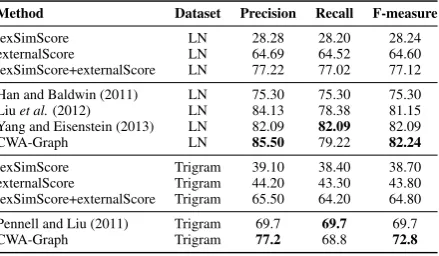
The results obtained by our proposed Contex-tual Word Association Graph (CWA-Graph) sys-tem on the LexNorm1.1 and trigram datasets, as well as the results of recent studies that used the same datasets for evaluation are presented in Ta-ble 5. The ill-formed words are assumed to have been pre-identified in advance.

Method Dataset Precision Recall F-measure

lexSimScore LN 28.28 28.20 28.24

externalScore LN 64.69 64.52 64.60

lexSimScore+externalScore LN 77.22 77.02 77.12

Han and Baldwin (2011) LN 75.30 75.30 75.30

Liuet al.(2012) LN 84.13 78.38 81.15

Yang and Eisenstein (2013) LN 82.09 82.09 82.09

CWA-Graph LN 85.50 79.22 82.24

lexSimScore Trigram 39.10 38.40 38.70

externalScore Trigram 44.20 43.30 43.80

lexSimScore+externalScore Trigram 65.50 64.20 64.80

Pennell and Liu (2011) Trigram 69.7 69.7 69.7

CWA-Graph Trigram 77.2 68.8 72.8

Table 5: Results obtained when ill-formed words are assumed to have been pre-identified in ad-vance.

Our CWA-Graph approach achieves the best F-measure (82.24%) and precision (85.50%) among the recent previous studies. The high precision value is obtained without compromising much from recall (79.22%). Our recall is the second best among others. The F-score (82.09%) obtained by Yang and Eisenstein (2013)’s system is close to ours and the second best F-score, which on the other hand, has a lower precision.

Without any modification to our system or to the parameters, we were able to improve the re-sults obtained by Pennell and Liu (2011) on the trigram SMS-like dataset. The trigram nature of the dataset resulted in input texts which are (short thus) very limited with regard to contextual infor-mation. Nevertheless, our system achieved72.8%

F-Measure using this contextual information even though it is limited.

Along the systems (presented in Table 5) that assume ill-formed tokens have been pre-identified

perfectly by an oracle, there are also systems that are not based on this assumption but contain ill-formed word identification components (Han et al., 2012; Hassan and Menezes, 2013; Chrupala, 2014). We used the method described in Section 4.4 to identify the candidate tokens for normaliza-tion. Table 6 shows our results compared with the results of other systems that perform ill-formed word detection prior to normalization. We could label 1141 tokens correctly as ill-formed among 1184 ill-formed tokens. We achieved a word error rate (WER) of 2.6%, where Chrupala (2014) re-ported 4.8% and Han et al. (2012) rere-ported6.6%

WER on the Lexnorm1.1 dataset.

Method Dataset Precision Recall F-measure

Han et al. (2012) LN 70.00 17.90 28.50

Hassan and Menezes (2013) LN 85.37 56.40 69.93

CWA-Graph LN 85.87 76.52 80.92

Table 6: Results obtained without assuming that ill-formed words have been pre-identified.

As shown in Table 5 some systems have equal precision and recall values (Yang and Eisenstein, 2013; Han and Baldwin, 2011; Pennell and Liu, 2011). Those systems normalize all ill-formed words. On the other hand, our system does not return a normalization, if there are no candidates that are lexically similar, grammatically correct, and contextually close enough. For this reason, we managed to achieve a higher precision com-pared to the other systems. Our system returns a normalization candidate for an OOV word only if it achieves a similarity score (contextual, lexical, external, or some degree of each feature) above a threshold value. The default threshold used in the system is set equal to the maximum score that can be obtained by lexical features. Thus, we only re-trieve candidates that obtain a non-zero contextual similarity score (conSimScore). The results shown at Table 7 and Table 8 demonstrate that CWA-Graph can obtain even higher values of precision by increasing the percentage of contextual context of candidates. It achieved94.1% precision on the LexNorm1.1 dataset, where the highest precision reported at the same recall level is85.37% (Hassan and Menezes, 2013). The precision of the normal-ization system can be set (e.g. as high, medium, low) depending on the application where it will be used.

conSimScore> Precision Recall F-measure

0 85.5 79.2 82.2

0.1 88.8 75.1 81.4

0.2 91.1 72.8 80.9

0.3 92.3 67.6 78.0

0.5 94.1 56.4 70.5

Table 7: Comparison of results for different threshold values on LexNorm1.1, the setup we have used for our other experiments is shown in bold.

conSimScore> Precision Recall F-measure

0 77.2 68.8 72.8

0.1 80.9 65.8 72.6

0.2 84.2 60.8 70.6

0.3 87.6 54.6 67.3

0.4 89.5 47.1 61.7

0.5 90.8 42.1 57.6

Table 8: Comparison of results for different threshold values on trigram dataset, the setup we have used for our other experiments is shown in bold.

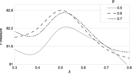
of the minor features compared to our major fea-tures (described in Sections 3.3 and 3.4). For the experiments reported in Tables 5, 6, 7 and 8 we set theλandβvalues to0.5. We did not tune these pa-rameters for optimized performance. Rather, our aim was to give less weight (half weight) to the minor features compared to the major ones. To analyze the effects of the lambda and beta param-eters, we plotted the performance of the system on the LexNorm1.1 data set by varying their values (see Figure 4). It is shown that forλandβvalues greater than0.3 the performance of the system is quite robust. The F-score varies between 80.4% and 82.9%.

Figure 4: The effect ofλandβ on the system per-formance.

5 Conclusion

In this paper, we present an unsupervised graph-based approach for contextual text normalization. The task of normalization is highly dependent on understanding and capturing the dynamics of the informal nature of social text. Our word associ-ation graph is built using a large unlabeled social media corpus. It helps to derive contextual analy-sis on both clean and noisy data.

It is important to emphasize the difference be-tween corpus based contextual information and contextual information of the input text (input con-text). Most recent unsupervised systems for text normalization only make use of corpus based con-text information. However, this approach is led by statistical information. In other words, it finds which IV word the OOV word is commonly nor-malized to, regardless of the context of the OOV word in the input text message. A major strength of our approach is that it utilizes both corpus based contextual information and input based contextual information. We use corpus based statistical infor-mation to connect/associate the words in the con-textual word association graph. On the other hand, the neighbors of an OOV word in the input text provide us input based context information. Using input context to find normalizations helps us iden-tify the correct normalization, even if it is not the statistically dominant one.

We compared our approach with the recent social media text normalization systems and achieved state-of-the-art precision and F-measure scores. We reported our results on two datasets. The first one is the standard text normalization dataset (Lexnorm1.1) derived from Twitter. Our results on this dataset showed that our system can serve as a high precision text normalization sys-tem which is highly preferable as an NLP pre-processing step. The second dataset we tested our approach is a SMS-like trigram dataset. The tests showed that the proposed system can perform good on SMS data as well.

The system does not require a clean corpus or an annotated corpus. The contextual word asso-ciation graph can be built by using the publicly available social media text.

References

Nor-malization. Proceedings of the 21st International Conference on Computational Linguistics and 44th Annual Meeting of the Association for Computa-tional Linguistics, pages 33–40.

Timothy Baldwin and Marco Lui. 2010. Language Identification: The Long and the Short of the Matter.

Human Language Technologies: The 2010 Annual Conference of the North American Chapter of the

Association for Computational Linguistics, pages

229–237.

Eric Brill and Robert C. Moore. 2000. An Improved Error Model for Noisy Channel Spelling Correction.

Proceedings of the 38th Annual Meeting on Associa-tion for ComputaAssocia-tional Linguistics, pages 286–293. Monojit Choudhury, Rahul Saraf, Vijit Jain, Animesh Mukherjee, Sudeshna Sarkar, and Anupam Basu. 2007. Investigation and Modeling of the Structure of Texting Language.International Journal on

Doc-ument Analysis and Recognition, 10(3):157–174.

Grzegorz Chrupala. 2014. Normalizing tweets with edit scripts and recurrent neural embeddings. Pro-ceedings of the 52st Annual Meeting of the Associa-tion for ComputaAssocia-tional Linguistics, pages 680–686. Danish Contractor, Tanveer A. Faruquie, and L. Venkata Subramaniam. 2010. Unsuper-vised Cleansing of Noisy Text. Proceedings of the 23rd International Conference on Computational Linguistics: Posters, pages 189–196.

Paul Cook and Suzanne Stevenson. 2009. An Un-supervised Model for Text Message Normalization.

Proceedings of the Workshop on Computational Ap-proaches to Linguistic Creativity, pages 71–78. Jacob Eisenstein. 2013. What to Do About Bad

Lan-guage on the Internet. Proceedings of the North American Chapter of the Association for

Computa-tional Linguistics : Human Language Technologies,

pages 359–369.

Kevin Gimpel, Nathan Schneider, Brendan O’Connor, Dipanjan Das, Daniel Mills, Jacob Eisenstein, Michael Heilman, Dani Yogatama, Jeffrey Flanigan, and Noah A. Smith. 2011. Part-of-speech Tagging for Twitter: Annotation, Features, and Experiments.

Proceedings of the 49th Annual Meeting of the Asso-ciation for Computational Linguistics: Human Lan-guage Technologies: Short Papers - Volume 2, pages 42–47.

Stephan Gouws, Donald Metzler, Congxing Cai, and Eduard Hovy. 2011. Contextual Bearing on Lin-guistic Variation in Social Media. Proceedings of

the Workshop on Languages in Social Media, pages

20–29.

Bo Han and Timothy Baldwin. 2011. Lexical Normal-isation of Short Text Messages: Makn Sens a

#Twit-ter. Proceedings of the 49th Annual Meeting of the

Association for Computational Linguistics: Human

Language Technologies - Volume 1, pages 368–378.

Bo Han, Paul Cook, and Timothy Baldwin. 2012. Au-tomatically constructing a normalisation dictionary for microblogs. Proceedings of the 2012 Joint Con-ference on Empirical Methods in Natural Language Processing and Computational Natural Language

Learning, pages 421–432.

Hany Hassan and Arul Menezes. 2013. Social Text Normalization Using Contextual Graph Ran-dom Walks. Proceedings of the 51st Annual Meet-ing of the Association for Computational LMeet-inguis- Linguis-tics, pages 1577–1586.

Max Kaufmann and Jugal Kalita. 2010. Syntactic Nor-malization of Twitter Messages. Proceedings of the 8th International Conference on Natural Language Processing, pages 149–158.

Vladimir Iosifovich Levenshtein. 1966. Binary Codes Capable of Correcting Deletions, Insertions and Re-versals. Soviet Physics Doklady, 10:707.

Fei Liu, Fuliang Weng, and Xiao Jiang. 2012. A Broad-Coverage Normalization System for Social Media Language. Proceedings of the 50th Annual Meeting of the Association for Computational

Lin-guistics: Long Papers-Volume 1, pages 1035–1044.

Marco Lui and Timothy Baldwin. 2012. Langid.Py: An Off-the-shelf Language Identification Tool. Pro-ceedings of the 50th Annual Meeting of the Associa-tion for ComputaAssocia-tional Linguistics: System Demon-strations, pages 25–30.

I. Dan Melamed. 1999. Bitext Maps and Alignment via Pattern Recognition. Computational Linguistics, 25(1):107–130.

Olutobi Owoputi, Brendan O’Connor, Chris Dyer, Kevin Gimpel, Nathan Schneider, and Noah A. Smith. 2013. Improved Part-of-Speech Tagging for Online Conversational Text with Word Clusters.

Proceedings of the North American Chapter of the Association for Computational Linguistics : Human

Language Technologies, pages 380–390.

Deana Pennell and Yang Liu. 2011. A Character-Level Machine Translation Approach for Normal-ization of SMS Abbreviations. Fifth International

Joint Conference on Natural Language Processing,

pages 974–982.

Deana Pennell and Yang Liu. 2014. Normalization of informal text. Computer Speech & Language, 28(1):256 – 277.

Lawrence Philips. 2000. The Double Meta-phone Search Algorithm. C/C++ Users Journal, 18(6):38–43, June.

Richard Sproat, Alan W. Black, Stanley Chen, Shankar Kumar, Mari Ostendorf, and Christopher Richards. 2001. Normalization of Non-Standard Words.

Computer Speech & Language, 15(3):287–333. Kristina Toutanova and Robert C. Moore. 2002.

Pro-nunciation Modeling for Improved Spelling Correc-tion. Proceedings of the 40th Annual Meeting on As-sociation for Computational Linguistics, pages 144– 151.

Yi Yang and Jacob Eisenstein. 2013. A Log-Linear Model for Unsupervised Text Normalization. Pro-ceedings of the Empirical Methods on Natural

Lan-guage Processing, pages 61–72.

Jaewon Yang and Jure Leskovec. 2011. Patterns of Temporal Variation in Online Media. Proceedings of the Forth International Conference on Web Search