Conical diffraction and the dispersion surface of hyperbolic metamaterials

Conical diffraction and the dispersion surface of hyperbolic metamaterials

K. E. Ballantine, J. F. Donegan, and P. R. Eastham School of Physics and CRANN, Trinity College Dublin, Dublin 2, Ireland

(Received 25 September 2013; revised manuscript received 6 May 2014; published 3 July 2014) Hyperbolic metamaterials are materials in which at least one principal dielectric constant is negative. We describe the refractive index surface, and the resulting refraction effects, for a biaxial hyperbolic metamaterial, with principal dielectric constants1<0, 0< 2=3. In this general case the two sheets of the index surface intersect, forming conical singularities. We derive the ray description of conical refraction in these materials and show that it is topologically and quantitatively distinct from conical refraction in a conventional biaxial material. We also develop a wave optics description, which allows us to obtain the diffraction patterns formed from arbitrary beams incident close to the optic axis. The resulting patterns lack circular symmetry and hence are qualitatively different from those obtained in conventional, positive index materials.

DOI:10.1103/PhysRevA.90.013803 PACS number(s): 42.25.Bs,42.25.Lc,78.20.Ci,78.67.Pt

I. INTRODUCTION

Hyperbolic metamaterials (HMMs), materials which have a negative dielectric constant in at least one direction, are attracting attention due to their interesting physics and myriad applications. They can be manufactured relatively simply from alternating layers of metal and dielectric, or by embedding metal rods in a dielectric background [1,2]. HMMs have recently been shown to have unique properties, described by effective medium theory [3], including a broadband infinite density of states [4], arbitrarily large values of the wave vector [5], and negative refraction [2,6]. This has led to many proposed applications, from imaging [7,8], sensing [9], and wave guiding [10,11] to information processing [12].

The most common HMMs considered are uniaxial mate-rials for which 1<0< 2=3 where i are the principal dielectric constants. This leads to a hyperboloid isofrequency surface (refractive index surface) for the extraordinary ray. The change in topology from an ellipsoid to a hyperboloid is responsible for many of the important properties of these materials [13]. The general case, however, is a biaxial HMM, where1<0< 2 < 3. Such a material could be realized as layers of metal and dielectric, where the dielectric material has uniaxial isotropy in the plane, or as rods of metal embedded in a dielectric with different rod spacings in the x and

y directions [14]. The isofrequency surface for the extraor-dinary ray is then an asymmetric hyperboloid [15].

In this paper we present the full two-sheeted isofrequency surface of a HMM, which describes the propagation of both the ordinary and the extraordinary rays with orthogonal polarizations, and show that it contains conical singularities. These singularities are degenerate points where the two sheets intersect at a point ink space. Similar conical singularities occur in conventional biaxial materials, i.e., 0< 1< 2<

₃[16,17], and lead to the phenomenon of conical refraction, in which a beam of light is refracted into two concentric hollow cones [17,18]. We describe these intersections in the case of a HMM and derive a geometrical optics description of refraction for rays with wave vector close to the degeneracy, including establishing the polarization and the Poynting vector, or energy flow. This predicts refraction into two intersecting rather than concentric cones, an effect topologically distinct from that in a conventional biaxial crystal and completely

lacking from a uniaxial HMM. We then extend this theory to develop a paraxial wave optics description of the propagation of light through these materials. This allows us to calculate the diffraction patterns formed from arbitrary beams incident on a biaxial HMM close to the optic axis. We find these patterns to be qualitatively different from those obtained in positive index materials, in particular lacking circular symmetry.

These conical singularities are, in some respects, similar to the Dirac points [19] that are of growing importance in solid-state physics. These points, where bands cross linearly at a particular frequency and wave vector, are best known in graphene [20,21]. Graphene has attracted huge theoretical and applied interest [22–24], with many new features attributable to the linear dispersion near a Dirac point, which means that the low-energy excitations are massless chiral Dirac fermions [21]. They thus provide a model of quantum electrodynamics with the limiting speed given by the Fermi velocity rather than the speed of light [21,25]. They also lead to effects such as the anomalous integer quantum Hall effect [26,27] and mean that electrons are immune to localization, propagating over large distances without scattering [20,28] . Tilted Dirac cones, which are not circularly symmetric around the degenerate wave vector, are similar to the skewed-cone intersections reported here and have previously been predicted in mechanically deformed graphene [29]. Dirac points in optical systems have been found in photonic crystals, as a result of the same lattice symmetry [30,31], or in materials with a frequency dependent permittivity, which may pass through zero at a particular frequency, leading to a degeneracy [32–34].

In these cases, however, a degeneracy occurs at a particular frequency, due to fine tuning the frequency to match the sublattice periodicity, or to match a zero of the frequency dependent dielectric constant. At other nearby frequencies there is generally no singularity. In contrast, biaxial materials have conical singularities in the isofrequency surface in

the dispersion relation (which describes a three-dimensional surface in the four-dimensional space ofωandk).

The remainder of this article is structured as follows. In Sec. IIwe describe the two-sheeted dispersion surface in a biaxial HMM and compare it to the case of positive. In Sec.III we derive the ray optics description of refraction, for incident rays with initial wave vector close to the optic axis, in a biaxial HMM. In particular, we present the polarization and Poynting vector, i.e., the direction of energy flow, of the refracted rays. In Sec.IVwe extend the theory to include small absorption in the material and show explicitly that the conical intersections persist. In Sec. V we develop a wave optics description of propagation near the optic axis of a biaxial HMM and present the diffraction pattern formed with a Gaussian input beam. In Sec. VI we discuss further the connection between conical singularities in optics and singularities in solid-state band structures. We make an explicit connection between the conical singularities described here and Dirac points by reformulating the diffraction theory in terms of the paraxial wave equation. Finally, in Sec.VIIwe summarize our conclusions.

II. DISPERSION SURFACES

We can describe a nanostructured metamaterial in the effec-tive medium theory by a three-dimensional dielectric tensor

ij or by the principal dielectric constants,i, which are its components in the frame in which it is diagonal [35]. Effective medium theory describes the subwavelength patterning of different materials by an average anisotropic dielectric tensor according to the Maxwell-Garnett formulas [36]. Plane-wave solutions to Maxwell’s equations in the medium lead to the Fresnel equation for the refractive index:

i

iη2i

n2₋ i

=0, (1)

where η is a unit vector in the direction of the wave vector k [35]. The two solutions for n2 _{for a given direction η} form a two-sheeted dispersion surface [35], also known as an isofrequency surface or refractive index surface. At a fixed frequency, these surfaces give the phase velocity, or equivalently the wave vector magnitude, in the medium, for a given wave-vector direction. The ray or energy flow direction will be orthogonal to the dispersion surface at the point defined by that wave vector [37]. In the following we assume without loss of generality that1< 2< 3.

Figure 1 shows sections of the dispersion surfaces for a variety of materials. These surfaces are polar plots where the radial distance represents the refractive index experienced by a ray propagating in that direction inkspace. Equivalently, they are three-dimensional cuts of the full four-dimensional space ofωandk, taken at a constantω. In the approximation where the dielectric constants depend weakly on frequency, these surfaces will simply contract or expand asωis decreased or increased, respectively, meaning the critical points will trace out lines. Outside of this approximation the dispersion surface will change shape but the basic features will remain until the dielectric constants cross each other or zero. Hence, assuming a smooth dependence on frequency, there will always be a

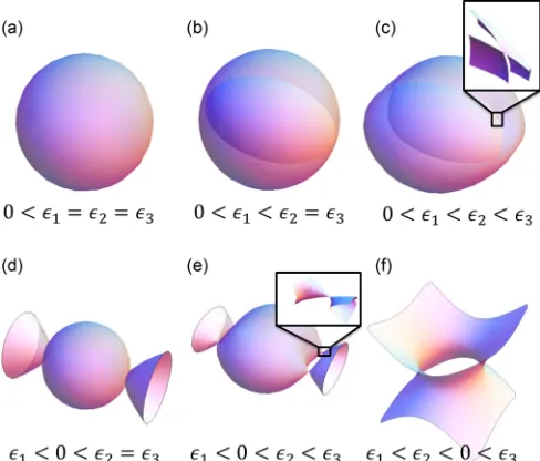
FIG. 1. (Color online) Isofrequency surfaces for various ef-fective index materials: (a) isotropic, (b) uniaxial, (c) biaxial, (d) uniaxial-hyperbolic, (e) hyperbolic type 1, and (f) biaxial-hyperbolic type 2. Shading is for perspective only. Additional cases not shown include1=2<0< 3, which is identical to (f) but with circular cross sections, and3<0, in which case there are no real solutions. These surfaces are polar plots of the refractive index as a function of ray directionη. In the case of (b) and (d) the surfaces intersect at two points, at which they are parallel. In the case of (c) and (e) the surfaces have four conical intersections. Insets in (c) and (e) show cutaway closeups of the intersection points. Cuts through these intersections are presented in Fig.2.

continuous range of frequencies for which these singularities exist.

The classical cases, 0< i, are shown in the first row and are the subject of conventional crystal optics. The surfaces have positive curvature and finite area. The hyperbolic cases, ₁<0, shown in the second row, are the result of nanostructured materials which have properties not found in nature at optical frequencies. They have dispersion surfaces which are unbounded in|k|at any frequency and feature both positive and negative curvature [1].

The possible classical materials fall into three categories. Figure 1(a) shows an isotropic material which has a single spherical dispersion surface. Once isotropy is broken, the surface splits into two as the two orthogonal polarizations experience different dielectric constants. For a uniaxial ma-terial, with two indices equal, these surfaces intersect at two points, along a single optic axis as shown in Fig.1(b). However, the surfaces are parallel at the degenerate points, and so the normals remain well defined [38]. For a biaxial crystal, shown in Fig.1(c), rotational symmetry is broken completely. The surfaces intersect at four points along two optic axes. The gradient of the surfaces is singular at the degenerate points and the normal is not well defined.

FIG. 2. (Color online) The transition from biaxial to biaxial-hyperbolic type 1 material as1passes through zero. One of the dispersion surfaces changes topology from an ellipsoid to a hyperboloid. The intersection points move from thex-zplane to thex-yplane. The first row shows the surfaces in thex-zplane (y=0). The second row shows the surfaces in thex-yplane (z=0).

wave vectors, called the ordinary and extraordinary rays. In conical refraction, when the incident wave vector coin-cides with the optic axis, the two orthogonally polarized incident rays are refracted into two concentric cones which contain all polarizations at different points around each cone [18,35].

When one of the dielectric constants becomes negative, leading to a hyperbolic metamaterial, there is a topological transition of one of the surfaces, from an ellipsoid to a hyperboloid. Figure1(d)shows a uniaxial HMM. The surfaces again intersect at two points where they are parallel. In the case of a biaxial HMM, shown in Fig.1(e), linear crossings occur. The hyperboloid and the ellipsoid intersect at four degenerate points. We describe for the first time these conical singularities in the dispersion surface of a biaxial HMM, and their associated refraction and diffraction effects. In the final case, where two of the three indices are negative, Fig.1(f), there is again a single dispersion surface which is a type two hyperboloid [1] with no singularities. This single dispersion surface describes one polarization which can propagate in the material. For the orthogonal polarization the material is metallic, and absorbing, and hence there is no second real solution to the Fresnel equation.

In both Figs.1(b)and1(d)the two sheets have a quadratic degeneracy. Including the perturbation ₂=₃ will clearly either open a gap or cause the quadratic intersection to split into two linear intersections, in line with general band theory. If a gap were to open, however, it would leave at least one closed surface which described the propagation of a different linear polarization at each point. The field of polarization directions described by this surface would form a tangential vector field on a closed two-dimensional surface. This is forbidden by the hairy ball theorem, unless the linear polarization vanishes at least once. Comparing with the Poincar´e sphere representation for the polarization, we see that such points, if they occurred, would correspond to points with circular polarization. However, in the presence of chiral symmetry the two circular polarizations cannot have different refractive indices, so that there cannot be a gap at these points. Thus, in the presence of chiral symmetry, the existence of conical singularities in the isofrequency surface is required on topological grounds. In its absence, however, a gap does indeed appear [39].

The transition from a conventional biaxial material to a biaxial type 1 HMM is shown in Fig.2as1goes from positive to negative. As rotational symmetry in they-zplane is broken (note we use the subscriptto denote the basis in whichis diagonal), the degenerate points are free to move around the

x axis as 1 varies. The points start in thex-z plane and move closer to thexaxis as1→0. Then as the topological transition occurs the critical points change direction and move away from thexaxis into thex-yplane.

The topological transition between the conical singularities of positive and negative index materials can be seen by calculating the solutions to the Fresnel equation, Eq. (1), which are degenerate. We find two sets of solutions:

η1= ±

3(2−1)

2(3−1)

,

η₂=0, (2)

η₃= ±

1(3−2)

2(3−1) and

η1= ±

2(3−1)

3(2−1)

,

η2= ±

−1(3−2)

3(2−1)

, (3)

η3=0.

The first solution Eq. (2) is real, and therefore physical, when all the i are positive. As1 becomes negative, η3 in Eq. (2) becomes imaginary. The second solution, Eq. (3), then becomes the real, physically relevant,η. In this way the transition through1=0 separates topologically distinct sets of degenerate solutions.

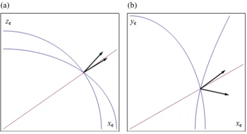
FIG. 3. (Color online) Cross sections of the isofrequency sur-faces through the degenerate points for (a) a conventional biaxial material and (b) a hyperbolic biaxial material. The optic axis is shown by the straight line, and the approximate normals to the surfaces for akvector passing close to this axis are shown by the arrows and are suggestive of the expected conical refraction. In the hyperbolic case the cone points toward rather than away from thexaxis.

approximately coincide with the optic axis. In the positive

case, one points close to the optic axis while the other points away from the x axis. In the case of a biaxial HMM the surfaces have opposite curvatures. This leads to one of the normals pointing towards the x axis. When the full two-dimensional surface is considered, the normals shown here contribute to a cone which is skewed away from the optic axis, in a different direction in each case. In Fig.3(b), one of the normals points downward, below the horizontal. If the material is cut so the interface is they-zplane, i.e., the normal is parallel to thexaxis, then this results in part of the cone being refracted back on the same side of the normal to the incoming ray, a phenomenon sometimes known as negative refraction. However, this term is also used to refer to negative phase velocity, which is not present in this case.

III. GEOMETRICAL OPTICS

We now turn to describing the refraction of light incident on a biaxial HMM, when the incident wave vector lies close to the optic axis, as shown in Fig.3. To achieve this we calculate the refractive index surface experienced by the ray and the resulting Poynting vector of the refracted ray. We describe the ray by polar coordinates in a frame where thexaxis coincides with the optic axis, and thezaxis coincides with thezaxis, as illustrated in Fig.4.θis the angle between the ray and the optic axis, whileφ is the azimuthal angle from they axis in they-z(transverse) plane. Expressingηin terms ofθandφ

and solving Eq. (1) we find the refractive index to first order inθis

n2=3−θ δ(cosφ±1), (4) where

δ =3

(3−1)(2−3)

12

(5)

is a measure of the anisotropy of the medium. The surface described by Eq. (4) consists of two cones touching at their points, which is the linear approximation to the surface

FIG. 4. (Color online) The coordinate system used to describe refraction near the optic axis in a biaxial HMM. The x axis corresponds to the optic axis through the direction given by Eq. (3) while the z axis corresponds to the z axis. θ is the angular displacement of the ray from the optic axis whileφis the azimuthal angle of the ray in the transverse plane.

portrayed in Fig.1(e) around one of the intersection points. Furthermore, we find the polarization of the two refracted rays is

Dz

Dy

= sinφ

cosφ±1, (6) whereDis the electric displacement field.

The results, Eqs. (4) and (6), describe the refractive index experienced by an incoming ray. A ray which comes from an azimuthal angleφcan be decomposed into the two orthogonal polarizations given by Eq. (6). These two polarizations experi-ence the refractive indices given by Eq. (4). The polarizations are independent ofθ, as long asθis small. Thus, for any ray not exactly coincident with the optic axis, there are two distinct polarization modes. Asφvaries, the direction of polarization described by a given dispersion surface rotates, so that a ray with one linear polarization and azimuthal angleφundergoes the same refraction as a ray with the orthogonal polarization and azimuthal angleφ+180◦. However, Eq. (6) is undefined whenθ =0. Hence there is also a polarization degeneracy at the conical singularity where all polarizations experience the same refractive index.

Equation (4) differs from the usual case of conical refraction in a biaxial crystal in two noteworthy ways. First,3plays the role of the average dielectric constant, despite being the largest of the three indices, while for a conventional biaxial crystal the median index2plays this role. Second, the parameterδ depends on√3−1, which is a large parameter since1 is negative. In the conventional,i>0, case of conical refraction the corresponding form is δ =2

√

(2−1)(3−2)/13, which is usually small. The polarization modes given by Eq. (6) are identical to the positive case. Thus we do not expect the polarization profiles generated by conical refraction and diffraction to change.

We now calculate the Poynting vector using Eqs. (4) and (6) for the two orthogonal polarizations associated with each incident wave vector. The Poynting vector is, up to an overall constant, given by

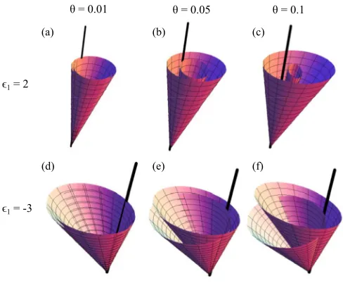
FIG. 5. (Color online) The loci of the Poynting vector of the two modes in a conventional biaxial material and a biaxial hyperbolic metamaterial, for wave vectors making anglesθandφto the optic axis, asφvaries from zero to 2π. In the conventional case the cones are concentric, while in the hyperbolic case they intersect. Forθ→0 the cones are degenerate. Asθ increases they move further apart. Parameters used are2=3 and3=4. Top row,1=2: (a)θ=0.01, (b)θ=0.05, and (c)θ=0.1. Bottom row,1= −3: (d)θ=0.01, (e)θ=0.05, and (f)θ=0.1. The solid black line indicates the optic axis, while the shading is for perspective only.

relations. The result,

Px = 1

₃3/2 +θ δ

₃5/2(cosφ±1),

Py =

δ

2₃5/2(1±cosφ)+

1

√

3

θ

±2δ

4₃3(cosφ±1)

2

(8)

+1

2

1

1

+ 1

2

(cosφ±1)∓ 1

3

,

Pz= ±

δ

25₃/2sin φ+√1

3

θ

_δ2

43₃(cosφ±1) sinφ

+1

2

1

1

+ 1

2

sinφ

,

is compared with thei>0 case in Fig. 5 for three values ofθ.

Equations (6) and (8) together describe the refraction of an incoming ray with wave vector at a small angleθto the optic axis and an azimuthal angleφin the perpendicular plane. Asφ

is varied, the resulting rays sweep out two intersecting cones while the polarization component which is refracted into each cone also varies. Forθ=0 a single ray of any polarization is refracted into a complete cone, containing all polarizations. However, any realistic incoming beam will be a superposition of rays with theθ=0 ray contributing an infinitesimal amount to the resulting pattern [18].

Figure5shows the loci of the Poynting vectors at different fixed anglesθas the azimuthal angleφis varied, for a biaxial

conventional material and a biaxial HMM. This is indicative of the paths taken by refracted rays in the material. The figures show that the usual result of two concentric cones [18] changes to the topologically distinct case of two intersecting cones. At

θ ≈0 the cones are degenerate and skewed away from the optic axis. The degeneracy is clear from Eq. (8). Forθ=0 the terms which depend onφtake the same value for one mode at a givenφas for the other mode atφ+π. Asθincreases, the cones move in opposite directions along theyaxis, so that they intersect and for large enoughθwill separate entirely. We note that this is due to a particular term in the Poynting vector, Eq. (8),

Py ∝ · · · +θ

1 2

1

₁ +

1

₂

(cosφ±1)∓ 1

₃

, (9) which is the dominant term for the movement of the cones asθ

increases. For1≈ −2, the first term in Eq. (9) is small, and so the two modes have terms≈∓θ/3inPyof opposite sign with little dependence onφ. This means the entire cones will move in opposite directions asθincreases. There is a corresponding term in the conventional case, but there if₁≈₂≈₃it is the constant terms±1/21±1/22∓1/3 which approximately cancel, leaving a term which is dominated by cosφ. Thus the centers of the cones do not move in this case.

IV. ABSORPTION

So far it has been assumed that although the permittivity may be negative it will always be real. Since hyperbolic metamaterials contain a large proportion of metal, they will always have some absorption, leading to an imaginary part of the effective permittivity. Although metals generally have high absorption, it is possible to design hyperbolic metamaterials with a small imaginary part ofover a range of frequencies [3]. Nevertheless it is important to consider how losses will affect the basic theory. Previous figures have plotted the real solutions of the Fresnel equation. In directions in which only one real solution exists, the other solution is completely imaginary and thus evanescent. When the permittivity is complex, all solutions are complex and represent waves which travel with some absorption, which depends on the size of the imaginary component.

3 2 1 1 2 3 y

3 2 1 1 2 3x

0 1

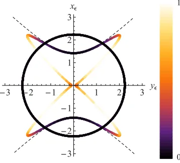
FIG. 6. (Color online) Isofrequency surface in the x-y plane (z=0) showing conical intersection in the presence of loss, with 1= −2+0.3i,2=2+0.3i, and 3=5+0.3i, similar to the bottom right panel of Fig.2. This is a polar plot of the real part of the refractive index with direction, with color representing the imaginary part of the refractive index, i.e., the absorption. White represents solutions with large absorption, and black represents those which are fully propagating. The original intersection remains a mostly propagating solution. An additional intersection appears which is mostly imaginary. The inclusion of an imaginary component to the effective medium theory is enough to prevent the dispersion surface becoming infinite. The dashed line shows the continuation of hyperbola in case of real.

We also note, from Fig. 6, that in the case of complex dielectric constants the refractive index no longer goes to infinity: the open hyperboloid becomes closed and finite. This is purely a result of including losses, without leaving the effective medium theory. The hyperboloid dispersion surface bends back at finitek, intersecting the ellipsoidal surface again. This second intersection has a large imaginary component, meaning that rays in this direction will decay quickly. These new intersections also occur in other directions ofη, where they are also mainly evanescent. As the imaginary component ofis increased, this finite hyperboloid shape will decrease in size, until the mostly real and mostly imaginary intersections approach each other and finally disappear. However, mostly imaginary intersections also appear in the x-z plane and remain for large imaginary components, in keeping with our previous topological argument.

V. DIFFRACTION

A complete treatment of optics near the conical singularities in a HMM must allow for diffraction of the incident and refracted beams. Here we develop such a treatment and obtain formulas for the diffraction patterns generated by arbitrary beams, incident on a biaxial HMM, with wave vectors close to the optic axis. We follow the method of [17]; in particular we use the angular spectrum representation to calculate the contribution of each input ray to the beam at a fixed propagation distance. Describing beams propagating close to the optic axis, which we will continue to label as thex axis, the field at a position x in the crystal consists of a sum of

plane-wave components which pick up a phase on propagating:

Eout=

dkydkzEin(ky,kz) exp[i(kyy+kzz)]

×exp ix

k2

T −ky2−k2z

, (10)

whereEin(ky,kz) is the two-dimensional Fourier transform of the input field in the planex =0. However, the magnitude of the total wave vector in the crystal kT is nk0, with n depending on the direction of the ray, i.e., onkyandkz. We can express the refractive index given by Eq. (4) in terms of the relative transverse momentum p=k_⊥/k, where k= √₃k₀

is the magnitude of a wave vector lying directly along the optic axis. For smallθ the transverse momenta are related to the angles defined in Fig.4bypz=θsin(φ),py =θcos(φ), andp= |p| =θ. The lowest-order terms, linear inp, lead to refraction into a simple cone which dominates the diffraction pattern. To reveal the fine structure we expand to second order, giving

n2≈3−δ(py±p)+

p±

2 δ

₃py

(p∓py)

≡3[1+μ(py,p)], (11) where

=

₃2 12

(23−1−2). (12)

Lettingk2

T =n2k02=k2[1+μ(py,p)] we can expand the square root in the final exponent of Eq. (10), again toO(p2_), giving

k2

T −k2⊥=

n2_k2

0−k2p2

=k

1+μ(p,py)−p2

≈k 1+1

2μ(p,py)− 1

8μ(p,py) 2₋1

2p 2_,

(13) where we keep terms up toO(p2) inμ2.

The integral Eq. (10) with the approximation given in Eq. (13) gives the paraxial approximation to the electric field at a planex >0, valid for small transverse momentum

a point (x,r_⊥) can then be written as the sum of the diffracted intensities from each eigenpolarization:

I = |b₊|2+ |b₋|2. (14) Expressing Eq. (10) in terms ofpand using Eq. (13) gives

b_±(x,r_⊥)= k 2πe

ikx

d2p a(p) exp(ikp·r_⊥)

×exp

−ikp2[βl+1

2

√

₃(x−l)]

×exp −iklαp_y2

×exp[±iklp(γ+δpy)], (15) where a(p) is the Fourier transform of the input field and

α,β,γ, and δ are all expressed in terms of i; the explicit forms are given in the Appendix. These parameters control the diffraction patterns and have the following interpretations:

β is a propagation constant,γ is proportional to the angle of the cone opening, andαandδcontrol the fine structure of the diffraction pattern leading to circular asymmetry.

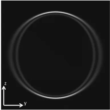
As a specific application of the diffraction formulas, Eqs. (14) and (15), we show in Fig. 7 the conical diffraction pattern formed for a Gaussian beam, a(p)=

kw2_exp(−k2_p2_w2_{/2). The beam waistwis taken as the unit} length scale. The resulting intensity profile is plotted in the focal image plane,x=l−2βl/√₃, where the resulting ring structure is sharpest. This position corresponds to the image of the input beam waist in an isotropic crystal of index√3, and the pattern here can be imaged with a lens if it occurs inside or before the crystal [17]. Asα,β,γ ,andδ all appear multiplied byl for propagation inside the crystal; the length of the crystal is only important relative to the overall scale of these parameters; e.g., a short, strongly diffracting crystal will have the same effect as a long, weakly diffracting one. The parameterγ l is chosen to give a ring radius r0≈50w to ensure well-developed rings while the other parameters are

FIG. 7. The intensity profile formed by conical diffraction of a Gaussian beam in a hyperbolic metamaterial, in the focal image plane (see text). The pattern is generated from the paraxial diffraction integral, Eq. (15), withαl=10 andδ=0.

αl =10,δl=0. This choice allows us to show the asymmetry of the beam on the same scale as the overall conical refraction. Like the positivecase, the diffraction pattern consists of two rings. In contrast to that case, however, the diffraction pattern is not circularly symmetrical. The rings are broadened in theydirection but remain tight in thezdirection. This is in agreement with Fig.5, which shows the cones moving apart in the y direction with increasingp. The diffraction pattern is bounded approximately on the inside and the outside by the arcs of two intersecting circles, also in agreement with the ray diagram. In addition there is a dark ring. This is purely an effect of diffraction and is not predicted by geometrical optics [18]. A similar dark ring, known as the Pogendorff ring, also appears in the conventional positivecase.

VI. DISCUSSION

As discussed in the introduction, a key feature of our results is the existence of linear intersections in the isofrequency surface in HMMs. These resemble the Dirac points that are of great interest in both condensed-matter physics and optics. It is therefore important to consider the relation between these phenomena carefully.

The dispersion surfaces describing the propagation of light in a biaxial material can be related to a band structure in two ways. The most straightforward is to consider the full dispersion relation ω(k) of light, which is a surface in the four-dimensional space ofωandk, and compare it with the corresponding dispersion relation for electrons in a periodic lattice. In this case, the isofrequency surfaces described here are directly equivalent to a constant energy surface like the Fermi surface, and not directly to the dispersion relation as usually plotted. Both are, of course, cross sections of the full dispersion relation in the four-dimensional space ofωandk, but in different directions.

For electrons there are two spin states related by time reversal, so that if time-reversal symmetry is presentω₊(k)=

ω₋(−k). If there is spatial inversion symmetry then we further-more haveω₋(k)=ω₋(−k). Hence if these two symmetries are present there is only one, doubly degenerate, sheet to the Fermi surface. This is a case of Kramer’s degeneracy. If one of these symmetries is broken then the spin-up and spin-down electrons can have different Fermi surfaces which may have conical intersections analogous to those described here, with the most common example being ferromagnetism [40].

For photons there are also two states, corresponding to the two polarizations, but these are related not by time-reversal symmetry, but by electromagnetic duality. This symmetry is present if the electric and magnetic fields can be interchanged. In most materials it is broken, because =μ, and this allows full frequency gaps to open, for example in a photonic crystal [41]. In terms of the isofrequency surfaces the (usual) breaking of this symmetry lifts the polarization degeneracy for most directions, leaving only the isolated point singularities described here.

we construct the paraxial Helmholtz equation describing conical diffraction in a biaxial HMM. We begin by writing the electric field as a plane wave times a slowly varying envelope function:

E(r)=A(r) exp(ikx), (16) whereA(r) varies slowly withx. The diffracted field given by Eq. (15) can be expressed as the two-dimensional transverse input field evolving in thexdirection as

E(r_⊥,x)=exp

−ik x

0

dxH(p,x)

E(r_⊥,0), (17) where for conical diffraction in a HMM we find that the Hamiltonian is

H=αp_y2+βp2+(γ+δpy)s·p (18) forx < land is the free Hamiltonianp2_{/2 forx > l. Heres=}

{σ₃,σ₁}is a vector of Pauli matrices in a Cartesian basis and pis formally represented by−i∇_⊥/k. The envelope function, thus, obeys the paraxial Helmholtz equation, which takes the form

H A= i k

∂A

∂x. (19)

Since this is equivalent to the Schr¨odinger equation [42], the propagation with x of the two-dimensional transverse beam is equivalent to the evolution with time of the wave function for a spin-1/2 particle. The birefringence of a biaxial material appears as a spin-orbit coupling, whose explicit form, close to the optic axis for a HMM, can be seen in Eq. (18). This form, with different definitions of the constants, also applies to a conventional biaxial material, but in that case the anisotropic terms proportional to α and δ are negligible and can be dropped [17].

Since light (of a fixed frequency) propagates in space according to Eq. (19), with x playing the role of time, the propagation constant kx can be interpreted as the energy. The isofrequency surfaces can thus be seen as a dispersion relation, giving the propagation constant as a function of the two transverse momentaky,kz. The point intersections in the isofrequency surfaces then correspond to Dirac points for two-dimensional electrons; specifically, the point intersections dis-cussed here are the Dirac points of the Hamiltonian, Eq. (18). Dirac points in two-dimensional materials have been of interest for their role in topological insulators and topologically protected edge states [43,44]. In a hexagonal lattice such as graphene, subject to time-reversal symmetry and spatial inversion symmetry, the electronic band structure must contain Dirac points. These degeneracies can be lifted by breaking spatial inversion symmetry, leading to a trivial insulator, or by breaking time-reversal symmetry, leading to a topolog-ical insulator [45]. Hence, work on topological effects in photonic systems has focused on Dirac points, primarily in the full frequency dispersionω(k) [41,46,47]. More recently,

however, attention has shifted to the analogous Dirac, or conical, intersections in the paraxial propagation constant surface [39,48,49]. Understanding the effects of different sym-metries on these two dispersion surfaces could therefore help progress toward topologically protected photonic systems.

VII. CONCLUSIONS

These results illustrate the unique singularities found in hyperbolic metamaterials when all three indices are allowed to vary independently. By examining the full dispersion surface of a general, biaxial, hyperbolic metamaterial, we have identi-fied conical singularities at which the refraction direction is not defined. We have found the approximate dispersion surface and the refracted Poynting vector for a ray traveling close to the axis of these singularities. We have shown that this leads to a new form of refraction which does not appear in the usual uniaxial HMMs and is topologically and quantitatively different from the phenomenon of conical refraction which occurs in ordinary biaxial materials. These propagating solutions remain when a small imaginary component is included, leading to a small amount of absorption, with additional mostly evanescent singular solutions also appearing. We have also calculated the diffraction pattern for a beam traveling through such a material. We have found that the diffracted beam is generally not circularly symmetric and that, similar to the positive

case, a dark ring appears where ray optics predicts the largest intensity.

ACKNOWLEDGMENTS

This work was supported by Science Foundation Ireland Grant No. SIRG I/1592 and by the Higher Education Authority under Programme for Research in Third-Level Institutions funding cycle 5. The authors wish to thank Prof. J. G. Lunney for useful discussions.

APPENDIX

We provide the parameters used in the diffraction theory in terms of the dielectric constants of the material:

α= δ

8 −

2 23

, β= 1

2(−1)+ 1 8δ,

(A1)

γ = 1

2δ, δ=

_δ2

23

+δ 4 −

2 , recalling from Eqs. (5) and (12) that

δ =3

(₃−₁)(₂−₃)

₁₂ ,

(A2)

=

2 3

₁₂(23−1−2).

[1] C. L. Cortes, W. Newman, S. Molesky, and Z. Jacob,J. Opt.14, 063001(2012).

[3] O. Kidwai, S. V. Zhukovsky, and J. E. Sipe,Phys. Rev. A85, 053842(2012).

[4] Z. Jacob, I. I. Smolyaninov, and E. E. Narimanov,Appl. Phys. Lett.100,181105(2012).

[5] X. Yang, J. Yao, J. Rho, X. Yin, and X. Zhang,Nat. Photon6, 450(2012).

[6] D. R. Smith, P. Kolinko, and D. Schurig,J. Opt. Soc. Am. B21, 1032(2004).

[7] Z. Jacob, L. V. Alekseyev, and E. Narimanov,Opt. Express14, 8247(2006).

[8] Z. Liu, H. Lee, Y. Xiong, C. Sun, and X. Zhang,Science315, 1686(2007).

[9] A. V. Kabashin, P. Evans, S. Pastkovsky, W. Hendren, G. A. Wurtz, R. Atkinson, R. Pollard, V. A. Podolskiy, and A. V. Zayats,Nat. Mater.8,867(2009).

[10] A. A. Govyadinov and V. A. Podolskiy,Phys. Rev. B73,155108 (2006).

[11] Y. He, S. He, J. Gao, and X. Yang,J. Opt. Soc. Am. B29,2559 (2012).

[12] G. A. Wurtz, R. Pollard, W. Hendren, G. P. Wiederrecht, D. J. Gosztola, V. A. Podolskiy, and A. V. Zayats,Nat. Nano.6,107 (2011).

[13] H. N. S. Krishnamoorthy, Z. Jacob, E. Narimanov, I. Kret-zschmar, and V. M. Menon,Science336,205(2012).

[14] J. Elser, R. Wangberg, V. A. Podolskiy, and E. E. Narimanov, Appl. Phys. Lett.89,261102(2006).

[15] J. Sun, J. Zeng, and N. M. Litchinitser,Opt. Express21,14975 (2013).

[16] M. V. Berry and M. R. Dennis,Proc. R. Soc. A459,1261(2003). [17] M. V. Berry,Journal of Optics A6,289(2004).

[18] D. L. Portigal and E. Burstein,J. Opt. Soc. Am.59,1567(1969). [19] P. R. Wallace,Phys. Rev.71,622(1947).

[20] K. S. Novoselov, A. K. Geim, S. V. Morozov, D. Jiang, Y. Zhang, S. V. Dubonos, I. V. Grigorieva, and A. A. Firsov,Science306, 666(2004).

[21] A. H. Castro Neto, F. Guinea, N. M. R. Peres, K. S. Novoselov, and A. K. Geim,Rev. Mod. Phys.81,109(2009).

[22] A. K. Geim and K. S. Novoselov,Nat. Mater.6,183(2007). [23] D. R. Cooper, B. D’Anjou, N. Ghattamaneni, B. Harack, M.

Hilke, A. Horth, N. Majlis, M. Massicotte, L. Vandsburger, E. Whiteway, and V. Yu,International Scholarly Research Notices

2012,501686(2012).

[24] S. Das Sarma, S. Adam, E. H. Hwang, and E. Rossi,Rev. Mod. Phys.83,407(2011).

[25] K. S. Novoselov, A. K. Geim, S. V. Morozov, D. Jiang, M. I. Katsnelson, I. V. Grigorieva, S. V. Dubonos, and A. A. Firsov, Nature (London)438,197(2005).

[26] V. P. Gusynin and S. G. Sharapov,Phys. Rev. Lett.95,146801 (2005).

[27] Y. Zhang, Y.-W. Tan, H. L. Stormer, and P. Kim,Nature (London)

438,201(2005).

[28] P. A. Lee and T. V. Ramakrishnan, Rev. Mod. Phys.57, 287 (1985).

[29] M. O. Goerbig, J.-N. Fuchs, G. Montambaux, and F. Pi´echon, Phys. Rev. B78,045415(2008).

[30] M. Plihal and A. A. Maradudin, Phys. Rev. B 44, 8565 (1991).

[31] O. Peleg, G. Bartal, B. Freedman, O. Manela, M. Segev, and D. N. Christodoulides,Phys. Rev. Lett.98,103901(2007). [32] L.-G. Wang, Z.-G. Wang, J.-X. Zhang, and S.-Y. Zhu,Opt. Lett.

34,1510(2009).

[33] X. Huang, Y. Lai, Z. H. Hang, H. Zheng, and C. T. Chan,Nat. Mater.10,582(2011).

[34] L. Sun, J. Gao, and X. Yang,Opt. Express21,21542(2013). [35] M. Born, E. Wolf, and A. Bhatia,Principles of Optics:

Electro-magnetic Theory of Propagation, Interference and Diffraction of Light(Cambridge University, Cambridge, 1999).

[36] G. A. Niklasson, C. G. Granqvist, and O. Hunderi,Appl. Opt.

20,26(1981).

[37] L. Landau, E. Lifshitz, and L. Pitaevskii, Electrodynamics of Continuous Media(Pergamon, New York, 1984).

[38] E. Hecht,Optics(Addison-Wesley, Reading, MA, 2002). [39] W. Gao, M. Lawrence, B. Yang, F. Liu, F. Fang, J. Li, and

S. Zhang,arXiv:1401.5448.

[40] R. A. de Groot, F. M. Mueller, P. G. van Engen, and K. H. J. Buschow,Phys. Rev. Lett.50,2024(1983).

[41] A. B. Khanikaev, S. Hossein Mousavi, W.-K. Tse, M. Kargarian, A. H. MacDonald, and G. Shvets,Nat. Mater.12,233(2013). [42] D. Dragoman and M. Dragoman,Quantum-Classical Analogies,

The Frontiers Collection (Springer, New York, 2004). [43] F. D. M. Haldane,Phys. Rev. Lett.61,2015(1988).

[44] C. L. Kane and E. J. Mele, Phys. Rev. Lett. 95, 146802 (2005).

[45] M. Z. Hasan and C. L. Kane, Rev. Mod. Phys. 82, 3045 (2010).

[46] S. Raghu and F. D. M. Haldane, Phys. Rev. A 78, 033834 (2008).

[47] T. Ochiai and M. Onoda,Phys. Rev. B80,155103(2009). [48] M. C. Rechtsman, Y. Plotnik, J. M. Zeuner, D. Song, Z. Chen,

A. Szameit, and M. Segev, Phys. Rev. Lett. 111, 103901 (2013).