ABSTRACT
LI, XIAOTONG. Effects of Loading and Target Locations on Age-Related Kinematic Differences – A Study Using Statistical Parametric Mapping. (Under the direction of Dr. Katherine Saul.)
Aging is frequently associated with skeletal muscle changes including sarcopenia,
abnormal activation patterns, and reduction in its contractile properties. The consequences of
these skeletal muscle changes result in diminished ability to perform common activities of
the daily living (ADL) in healthy aging. Difficulty with ADLs may be, in part, a consequence
of strength and stability deficits in the upper limb resulting in compensatory kinematic
movement. The goal of this thesis was to study age-related effects on shoulder kinematics for
forward reaching functional tasks related to ADL performance requiring both postural and
load demands.
We measured the kinematic trajectories of 10 healthy older adults (72.4±3.1 years) and 18 young adults (72.4±3.1 years) during reaching tasks under high and low postural and load conditions. We obtained shoulder joint angle and velocity trajectories for each task condition
employing a musculoskeletal model of the upper limb. Age group effects on the three
shoulder degrees of freedom were examined and compared to each other using statistical
parametric mapping (SPM) and discrete two sample t-tests to reveal the main effect of age.
Additional discrete two sample t-tests were conducted to examine the effect of load demand
on joint kinematics.
Our results indicated that older adults preferred to use more forward flexed and
adducted postures to initiate and terminate their movements compared to young adults under
adults to alter their postures to be more flexed similar to older adults. These results indicate
older adults modified their movement postures to compensate for their concerns for stability;
more forward flexed and adducted postures have been previously shown to provide greater
limb stiffness as well dexterity during upper extremity tasks.
SPM has recently been used in the field of biomechanics to improve the quality and
accuracy of statistical analyses by analyzing data of multiple dimensions and avoiding
several sources of bias compared to discrete analysis methods. One-dimensional SPM was
implemented in this study and produced results consistent with discrete analyses of extracted
values from the time spectrum. However, the SPM analyses also explicitly revealed temporal
information regarding portions of movement for which kinematic strategies differ, and
© Copyright 2015 Xiaotong Li
Effects of Loading and Target Locations on Age-Related Kinematic Differences – A Study Using Statistical Parametric Mapping
by Xiaotong Li
A thesis submitted to the Graduate Faculty of North Carolina State University
in partial fulfillment of the requirements for the degree of
Master of Science
Mechanical Engineering
Raleigh, North Carolina
2015
APPROVED BY:
_______________________________ ______________________________
Dr. Gregory Buckner Dr. Gregory Sawicki
BIOGRAPHY
This thesis is a summary of my graduate work. I completed my undergraduate studies at
the University of Toledo in the Department of Mechanical Engineering from 2008 to 2012. I
started my graduate studies in 2013 at the North Carolina State University in the Mechanical
and Aerospace Engineering Department under the direction of Dr. Katherine Saul. The
primary focus of the Movement Biomechanics Laboratory is to investigate the relationship
between musculoskeletal structure and function of the upper limb. Specifically, I have
dedicated my graduate work to understanding how aging plays a role in functional
performance of the upper limb, and to understanding and applying advanced statistical
ACKNOWLEDGMENTS
The work and accomplishments I have achieved through my master’s thesis work
would not have been possible if it were not for the support and advice of Dr. Katherine Saul,
my advisor. You have given me guidance throughout my master’s degree and you have set an
example of excellence as a researcher, mentor, and instructor. I would also like to thank my
thesis committee members for taking time out of their busy schedules to discuss and give me
feedback on my work. I would also like to thank Dr. Meghan Vidt, Anthony Santago and Dr.
Melissa Daly for their efforts in the data collection process for this project. Meghan and
Anthony have also helped me with any question I had about the experiments and study
preparations. Anthony provided me with useful feedback on my presentations and
meaningful discussions about my research.
I would like to give special thanks to Dr. Todd Pataky for taking the time to respond to
my emails and guide me through the learning process of SPM. Your help has made it
possible for me to learn and use SPM extensively in my research. This work would not have
been possible without the generous support of my funding source from the National Science
TABLE OF CONTENTS
LIST OF TABLES ...v
LIST OF FIGURES ... vi
LIST OF ABBREVIATIONS ... vii
CHAPTER 1 INTRODUCTION ...1
1.1Age-Related Muscle and Movement Changes ...1
1.2Musculoskeletal Modeling and Kinematic Analyses ...18
CHPATER 2 STATISTICAL PARAMETRIC MAPPING ...24
2.1Background of SPM and Developments ...25
2.2Application of SPM in Movement Change Evaluations ...35
CHAPTER 3 AGE-RELATED DIFFERENCES IN KINEMATIC STRATEGY AS INFLUENCED BY LOAD AND TARGET LOCATION ...39
3.1Introduction ...39
3.2Methods...42
3.3Results ...47
3.4Discussion ...56
CHAPTER 4 CONCLUSIONS AND FUTURE WORK ...62
4.1Conclusions ...62
4.2Recommendations for Future Research ...64
REFERENCES ...67
LIST OF TABLES
Table 1. Type I and Type II Muscle Fiber Properties. ...9
Table 2. Common Terminology Used to Define Movement Characteristics. ...12
Table 3. Summary of Participants’ Demographic Information ...43
LIST OF FIGURES
Figure 1. Skeletal Muscle Hierarchical Structure. ...4
Figure 2. Structure of the Sarcomere. ...5
Figure 3. Hill-Type Muscle Model of the Skeletal Muscle. ...6
Figure 4. Depiction of a Motor Unit; Twitch of Neural Activation of Skeletal Muscle. ...7
Figure 5. Force Length and Force Velocity Relationships. ...8
Figure 6. Pathway from Sarcopenia to Disability. ...10
Figure 7. Young and Older Adult Position, Velocity and Acceleration Profiles. ...13
Figure 8. Generating a Muscle-Driven Simulation of a Subject’s Motion with OpenSim. ...19
Figure 9. Computational Model of the Upper Extremity. ...20
Figure 10. Computation Model Degrees of Freedom and Axis Definition. ...21
Figure 11. Inverse Kinematics in OpenSim. ...22
Figure 12. General Procedures to Implement SPM. ...27
Figure 13. Random Field Theory Applied at Different Thresholds...35
Figure 14. Applications of SPM in Biomechanical Analyses...37
Figure 15. Experimental Setup and Task Definition. ...43
Figure 16. Low Postural Demand with Low Load Task Kinematics. ...51
Figure 17. Low Postural Demand with High Load Task Kinematics. ...52
Figure 18. High Postural Demand with Low Load Task Kinematics. ...53
Figure 19. High Postural Demand with high Load Task Kinematics. ...54
Figure 20. Elevation Plane Angular Velocity of all Reaching Tasks. ...55
LIST OF ABBREVIATIONS
ADL = activities of the daily living
CC = contractile component
CMC = computed muscle control
DOF = degrees of freedom
EC = Euler’s characteristic
EEG = electroencephalogram
EMG = electromyography
FDA = functional data analysis
fMRI = functional magnetic resonance imaging
FWE = family wise error
GLM = general linear model
GRF = Gaussian random field
MTU = muscle tendon unit
PCSA = physiological cross-sectional area
PEC = parallel elastic component
PET = positron emission tomography
RFT = random field theory
ROM = range of motion
RRA = residual reduction algorithm
SEC = series elastic component
CHAPTER 1: INTRODUCTION 1.1 Age-Related Muscle and Movement Changes
The muscular system has three major types of muscle tissue: cardiac muscle, smooth
muscle, and skeletal muscle. Skeletal muscle is the most significant component of the three
in that it accounts for 40 to 45% of the total body weight (Lorenz and Campello, 2012).
Skeletal muscle attaches to the skeleton through tendon, delivering strength and protection
through load distribution and shock absorption (Lorenz and Campello, 2012). Through the
interactions of skeletal muscle, tendon, and ligaments, forces are generated which enable
movement of the skeletal system. These generated forces and movements provide the ability
to complete activities of daily living (ADLs), functional tasks required for self-care and
independent living. With advancing age, a common consequence is a diminished ability to
perform ADLs due to a number of age-related skeletal muscle changes including sarcopenia,
abnormal neural activation patterns, and reductions in the contractile properties of the
skeletal muscle (Clark and Manini, 2010; Morley, 2012; Narici and Maffulli, 2010;
Rosenberg, 1997). These declines in skeletal muscle are the primary causes of frailty in older
adults, and thus is a major cause of disability and loss of independence.
Another critical function of skeletal muscle is postural control and maintenance (Lorenz
and Campello, 2012). The ability to properly control postures provides individuals with
stability in a variety of body configurations such as seating, standing, and walking (Wade and
Jones, 1997). The ability to properly control and maintain body configurations allows
individuals to complete stationary and dynamic functional tasks. Since older adults undergo
stability are challenged. Consequently, older adults tend to restrict themselves from activities
with debilitating physical consequences, and have declined ability to perform ADLs due to
fear of falling or injury (Arfken et al., 1994; Zijlstra et al., 2007; Murphy et al., 2002). To
compensate for these stability deficits during standing reaches, older adults have been
reported to adopt alternative movement strategies to maintain postural stability (Tsai and Lin,
2015; Liao and Lin, 2008; Prioli et al., 2006). However, it remains unclear what strategies
older adults use to maintain and control upper extremity stability. In younger adults, upper
extremity stability is maintained by regulating limb stiffness; anterior arm postures have been
shown to improve stability and dexterity (Trumbower et al., 2009; Perreault et al., 2001;
Chen et al., 2010). However, whether this strategy can be extended to older adults who have
altered strength and coordination is unclear, especially with regard to the variety of task
demands experienced in the performance of daily functional tasks.
The goal of this thesis is to explore the effects of aging on kinematic strategies for
functional tasks under conditions that may challenge postural stability. To do this, we must
first understand the physiology of muscle and its force-generating behavior, the effects of
aging on muscle, and the current understanding of movement changes with age. It should be
noted that the effects of aging on the structural and functional properties of skeletal muscle,
as well as on task performance in the elderly, need to be distinguished from the effects of
disuse and disease. In this study, we focus on the physiological and functional changes
1.1.1 Muscle Anatomy and Physiology
A muscle fiber is the basic cellular component of skeletal muscle. It is a multinucleated
cell and contains hundreds of myofibrils, composed of units called sarcomeres. Sarcomeres
are the fundamental contractile machinery of the muscle, which are arranged in a repeated
serial pattern along the length of the myofibrils. Sarcomeres are separated by Z-discs and
contain contractile proteins myosin (thick filament) and actin (thin filament). Elastic
filaments called titin are attached at the ends of the myosin filaments and connect these thick
filaments to the walls of the Z-discs. The contractile properties of these proteins are achieved
through the interactions of the heads of the myosin filaments as they attach to the actin
filaments, sliding past each other to create tension in the sarcomere. Contraction requires
energy in the form of ATP (i.e. adenosine tri-phosphate) to create and release the bonds
between the actin and myosin molecules. This process is called cross-bridge cycling. The
ability of the sarcomeres to produce force is regulated by the supply of calcium ions to the
proteins, by way of the electric signal delivered to the muscle. The electrical signal, or action
potential, is sent to the sarcolemma from a motor neuron which excites the muscle at the
neuromuscular junction (Lorenz and Campello, 2012). Figure 1 shows a simplified structure
Figure 1. Structure of the Sarcomere (Zatsiorsky and Boris, 2012).
Skeletal muscle is made up of bundles of these fibers, bounded by a tubular cellular
structure called sarcolemma along with a sheath of collagenous tissue known as the
endomysium. Muscle fibers are multi-nucleated cells, arranged in bundles bounded by
perimysium to make up muscle fascicles. Many muscle fascicles are bound together by the
sheath-like epimysium to compose the whole muscle. Skeletal muscle is attached to bones
via tendon, forming a single muscle-tendon unit (MTU) (Zatsiorsky and Boris, 2012; Lorenz
and Campello, 2012). Figure 2 shows a detailed depiction of skeletal muscle composition and
Figure 2. Skeletal Muscle Hierarchical Structure (Lorenz and Campello, 2012).
The functional unit of skeletal muscle is the motor unit. A motor unit consists of a
single motor neuron and all the skeletal muscle fibers that are innervated by it, and can be
excited to contract individually. The mechanical response produced in muscle due to an
isolated pulse stimulation of a motor nerve is a twitch. Force in the muscle can be modulated
by the frequency at which twitches occur (Lorenz and Campello, 2012). At higher
stimulation frequencies, a summation effect increases muscle force beyond that of a twitch,
with maximal fused force referred to as muscle tetanus. Figure 3 shows an illustration of a
motor unit (top) and an example of a twitch, twitch summation, and tetanus. Muscle force
can also be modulated through the mechanism of orderly recruitment. The phenomenon of
motor units are recruited first. As the amount of force needed increases, large motor units are
then recruited as well (Henneman et al., 1965).
Figure 3. Depiction of a Motor Unit (Top); Twitch, Twitch Summation, Unfused and Fused Tetanus of Neural Activation of Skeletal Muscle (Bottom) (Austin Community College, 2008; Cummings, 2001).
1.1.2 Mechanical Behavior of Muscle Contraction and Force Production
To model the mechanical behavior of muscle contraction, the widely adopted Hill-Type
Muscle Model (Hill, 1938) can be used (Figure 4). This model represents the tendons
attached at the ends of skeletal muscles as spring-like elastic components that are serially
connected (Series Elastic Components (SECs)). The contractile proteins of the myofibrils
(myosin, actin) are represented as the Contractile Component (CC), while the sarcolemma,
Parallel Elastic Component (PEC). The parallel and series elastic components produce
tension and store energy during stretching under active contraction or passive extension. To
release this stored energy, these elastic components relax to return to their original lengths
(Lorenz and Campello, 2012).
Figure 4. Hill-Type Muscle Model of the Skeletal Muscle (Hill, 1938; Lorenz and Campello, 2012).
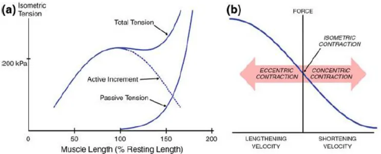
The total force generated by the skeletal muscle is the summation of the active forces
and passive forces generated by the muscle fibers (Gao and Leineweber, 2014). The active
forces are generated by the contractile proteins (myosin, actin) and the passive forces are
generated by the passive component when it is stretched beyond its resting length. These
passive components are the parallel elements in Hill’s model, and the magnitude of the
passive forces are a function of the material properties such as the passive elastic stiffness
(Gajdosik et al., 2005) of the tissues in the parallel elastic components.
Maximal active force is generated when muscle fibers are stretched to their optimal
length. At this length, the interactions between the myosin and actin are maximal and these
interaction. When muscle fibers are shortened, the active tension decreases with decreasing
length (Figure 5a). When the fibers are stretched beyond the optimal length, active force also
decreases due to the reduced cross-bridges possible between the myosin and actin filaments.
However, total force is the sum of both active and passive components, and when the muscle
is stretched past its optimal length, passive force increases markedly (Figure 5a) (Lorenz and
Campello, 2012; Gao and Leineweber, 2014). The amount of force generated in the muscle is
also related to the contraction velocity and the type of muscle contraction. During concentric
(shortening) contractions of the muscle, the amount of active force is reduced to zero at the
maximal shortening velocity. In contrast, as the muscle fibers lengthen during an active
contraction, active force increases with increased lengthening velocity of the muscle fibers
(Figure 5b) until muscle yielding.
Figure 5. Force Length and Force Velocity Relationships (Gao and Leineweber, 2014).
In addition to the optimal muscle length, the arrangement of the muscle fibers, or
muscle architecture, affects the functional properties of a particular muscle (Lieber, 2000). In
(e.g. vastus lateralis), or arranged in a multi-pennate pattern (e.g. gluteus) orienting in
multiple directions relative to its force-generating axis (Lieber, 2000). Based on this
arrangement, an important muscle architectural characteristic is the physiological
cross-sectional area (PCSA), describing the net cross-cross-sectional area of all muscle fibers within a
muscle. A larger pennation angle results in a larger PCSA (Lorenz and Campello, 2012). The
amount of force generated in the muscle is proportional to the PCSA, due to the larger
number of muscles fibers acting in parallel.
There are three main types of muscle fibers, as categorized by metabolic characteristics:
type I, slow twitch oxidative red fibers; type IIA, fast twitch oxidative-glycolytic red fibers;
and type IIB, fast twitch glycolic white fibers (Lorenz and Campello, 2012). Type I fibers are
characterized by slow contraction time and are resistant to fatigue due their oxidative
metabolism. Therefore, Type I fibers are recruited for movements where resistance to fatigue
is important. Type II fibers are characterized by fast contraction times and high susceptibility
to fatigue. These fibers are well suited to produce high forces quickly. Table 1 shows a
summary of the muscle fiber types and their corresponding characteristics.
Table 1. Type I and Type II Muscle Fiber Properties
Fiber Type Type I Type II
Contraction Speed Slow Fast
Activity Aerobic Anaerobic
Contraction Duration Long Short
Fatigue Properties Resistant to Fatigue
Prone to Fatigue
1.1.3 Age-Related Skeletal Muscle Changes
Aging is commonly associated with decreases in muscle mass (sarcopenia) and/or
muscle quality reduction (McDonagh et al., 1984; Clark and Manini, 2010; Morley, 2012:
Narici and Maffulli, 2010; Rosenberg, 1997). There are also associated alterations in neural
activation patterns, thus resulting in the decline in force production (Clark and Manini, 2010;
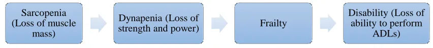
Hughes et al., 2001; Morley, 2012). Declined strength and muscle power (i.e. product of
muscle force and velocity) is called dynapenia and it is the direct cause for older adults to
become frailer with aging (Janssen, 2010; Morley, 2012). The pathway from sarcopenia to
the loss of functional ability and declines in the ability to perform ADLs has been modeled
by Morley (2012) (Figure 6). Note that the loss of muscle mass and quality can eventually
lead to disability and thus inability to perform ADLs. Therefore age-related strength and
muscle mass reduction can limit the independence of the elderly and possibly result in
disability.
Figure 6. Pathway from Sarcopenia to Disability (Adapted from Morley, 2012).
Changes in skeletal muscle occurs to both the active and the passive properties of
skeletal muscles. Changes in the active properties include muscle fiber type changes, muscle
fiber atrophy (reduced in size), and decreases in the number of muscle fibers (Larsson et al.,
1979; Narici and Maffulli, 2010; Narici et al., 2003). Larsson et al. have reported a decline in
Type II fibers of approximately 14.5% in older adults aged 60-65 when compared to young Sarcopenia
(Loss of muscle mass)
Dynapenia (Loss of
strength and power) Frailty
Disability (Loss of ability to perform
adults 20-29 years of age. The cross-sectional areas of Type I and Type II fibers also
declined significantly in the older age groups (approximately 23% to 42%, respectively)
(Larsson et al., 1979). Other researchers have also reported a preferential loss of fast twitch
motor units in older adults (Campbell et al. 1973).
Fiber architecture is also reported to alter with age, including decreases in both fiber
lengths and pennation angles (Narici et al., 2003). As a result, the shortening velocities and
force-generating capabilities in older adults decline with age. This is because shortening
velocity and force generating abilities of skeletal muscle are related to the number of
sarcomeres in series (fiber length), while the muscle’s peak force abilities are influenced by
the number of sarcomeres in parallel (i.e. muscle cross-sectional area) (Narici and Maffulli,
2010).
Altered passive muscle-tendon properties are also observed with age. Studies have
reported increased stiffness of the muscle’s extracellular matrix (endomysium, perimysium,
and epimysium) (Gao et al., 2008) and increases in collagen content in both endomysium and
perimysium (Gajdosik et al., 2005) with age. These findings indicate age-related alteration in
the passive stiffness of skeletal muscles which affects the range of motion during movements
(Gajdosik et al., 2005).
1.1.4 Functional Consequences and Movement Characteristics with Aging
The functional consequences of the aforementioned age-related musculoskeletal
changes are often associated with declined performance of functional tasks required for daily
living. Older adults have been reported to adopt alternative movement strategies in
2006; Morgan et al., 1994; Tsai and Lin, 2015; Liao and Lin, 2008). One method of
quantifying different strategies has been to evaluate altered movement kinematics during task
performance. The majority of studies performed to elucidate altered movement strategies for
upper limb movement employ target tracing/point experiments which track the endpoint
trajectories (e.g. fingertip) (Ketcham et al., 2002; Morgan et al., 1994; Darling et al., 1989).
Typical metrics to evaluate performance have included: total movement time (Ketcham et al.,
2002; Morgan et al., 1994); trajectory variability (Darling et al., 1989); range of motion
(Hortobágyi et al., 2003); peak endpoint velocity (Ketcham et al., 2002; Hortobágyi et al.,
2003; Darling et al., 1989); number of secondary movements (Ketcham et al., 2002; Morgan
et al., 1994); jerk (Ketcham et al., 2002); and muscle activation patterns (Darling et al.,
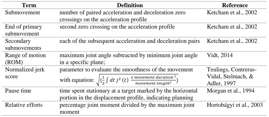
1989). Some terminologies commonly used to define upper limb kinematic characteristics
are tabulated in Table 2. Typical end-point position, velocity, and acceleration profiles for
young and old participants are depicted in Figure 7.
Table 2. Common Terminology Used to Define Movement Characteristics
Term Definition Reference
Submovement number of paired acceleration and deceleration zero crossings on the acceleration profile
Ketcham et al., 2002
End of primary submovement
second zero crossing on the acceleration profile Ketcham et al., 2002
Secondary submovements
each of the subsequent acceleration and deceleration pairs Ketcham et al., 2002
Range of motion (ROM)
maximum joint angle subtracted by minimum joint angle in a specific plane;
Vidt, 2014
Normalized jerk score
parameter to evaluate the smoothness of the movement
with equation: √(1
2∫ 𝑑𝑡 𝑗
2(𝑡) 𝑥 𝑚𝑜𝑣𝑒𝑚𝑒𝑛𝑡 𝑑𝑢𝑟𝑎𝑡𝑖𝑜𝑛 5 𝑚𝑜𝑣𝑒𝑚𝑒𝑛𝑡 𝑙𝑒𝑛𝑔𝑡ℎ2 )
Teulings, Contreras-Vidal, Stelmach, & Adler, 1997 Pause time time spent stationary at a target marked by the horizontal
portion in the displacement profile, indicating planning
Morgan et al., 1994
Relative efforts percentage joint moment divided by the maximum joint moment
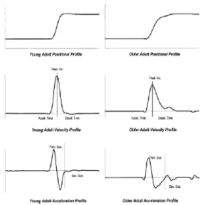
Figure 7. Young (Left) and Older (Right) Adult Position, Velocity and Acceleration Profiles. Older adults are characterized with less smooth movements (higher jerk scores);
asymmetrical velocity profiles (shortened acceleration phase and prolonged deceleration phase); and significantly more submovements compared to young adults. Tasks performed were target aiming tasks (Ketcham et al., 2002).Vel.: velocity, Accel.: acceleration, Decel.: deceleration , Prim. Sub.: primary submovement, Sec. Sub.: secondary submovement.
Studies employing endpoint tracking tasks often place emphasis on accuracy (Ketcham
et al., 2002; Morgan et al., 1994; Darling et al., 1989). In these studies, older adults were
reported to have a more flattened velocity profiles with a larger number of zero crossings (i.e.
multiple changes in the direction of velocity); slower movement velocities; smaller peak
velocities; shorter distances travelled during the primary submovement; more
submovements; and less smooth movements (marked by higher normalized jerk scores).
increased task difficulty and decreased target size (Ketcham et al., 2002; Morgan et al.,
1994). In general, for these accuracy tasks, older adults exhibited a shortened acceleration
phase and a prolonged deceleration phase in their velocity profiles (Figure 7), thus allowing
time to make corrective submovements. Therefore, movement asymmetry is often observed
in the movement profiles of older adults. Morgan et al. (1994) have suggested that no
significant time spent in the accelerating phase of the movement indicates that movement
slowing in older adults is not due to problems with force production; rather older adults
simply prefer to spend more time correcting their movements during the deceleration phase
to retain accuracy. That is, older adults are able to produce the necessary forces needed to
propel their limb to the target but the terminal accuracy requirements may be the cause of
difficulties in force modulating abilities (Ketcham et al., 2002). This emphasis on accuracy
(marked by the significant number of submovements) can also indicate a loss of certainty
during movements (Morgan et al., 1994). Darling et al. (1989) examined the acceleration and
deceleration profiles of older adults by studying trajectory variability (marked by movement
to movement variability) and how it changed with practice. They reported a significant
decrease in older adults’ trajectory variability as well as reduced asymmetry in their
movement profiles after extensive practice.
These kinematic differences were associated with altered muscle coordination. Darling
et al. (1989) have reported based on EMG recordings that older adults’ antagonist bursts
were inconsistent and often timed inappropriately, indicating mal-controlled activation
patterns. Increased cocontraction was shown prior to and during movements, which can
pattern may be associated with age-related muscle fiber type changes (Larsson et al., 1979).
Central planning deficits have also been reported as one of the causes for movement slowing;
these deficits can be the cause of abnormal coactivities including problems in timing and
phasing of muscle activation patterns (Hortobágyi et al., 2003; Darling et al., 1989). Another
possibility is that older adults have increased variability in motor unit discharge rate which
can result in skeletal muscle tension output variability during contraction, thereby increasing
the variability in movement endpoints (Darling et al., 1989). However, more consistent
activation patterns are observed with task practice in older adults (Darling et al., 1989),
resulting in a more stereotyped movement trajectory. Consequently, Darling et al. (1989)
have suggested that older adults can achieve the same or greater accuracies as young adults
after practice with only the constraint of lengthened movement durations.
The prior work in endpoint accuracy tasks suggests the importance of the experimental
protocol involved in elucidating possible kinematic differences. In particular, emphasizing
accuracy may compromise interpretation of the importance of differences observed in
kinematic patterns when functional performance during ADL tasks that do not require
accuracy is of interest. Further, familiarity with the task is important for evaluating typical
behavior, especially in older adults.
Another important requirement during older adults’ movement is their concern for
stability due to fear of falling and injury. Approximately 24%-54% of older adults experience
fear of falling (Zijlstra et al., 2007; Bruce et al., 2002; Murphy et al., 2002), and older adults
have been reported to adopt different movement strategies to increase stability and prevent a
as a measure to quantify full body stability with aging (Hageman et al., 1995; Norris and
Medley; 2011; Duncan et al., 1990; Tsai and Lin, 2015) and increased age has been
associated with deteriorated stability control capabilities. For example, a study between
young (mean age 23.7 years) and older females (mean age 70 years) found that when
instructed to reach forward with fast velocities, the reaching momentum and center of mass
velocity of the young females significantly increased compared to forward reaches at
comfortable speed, while that of the older females remained relatively unchanged. Young
females also inclined their trunk more compared to the older cohort (Kozak et al., 2003). This
is evidence that by limiting trunk flexion and reaching momentum, older adults adopted
different strategies to prevent a fall. In addition, when task demand was increased by means
of disturbing visual perception (Prioli et al., 2006; Hageman et al., 1995) and employing a
less stable standing surface (Norris and Medley, 2011; Prioli et al., 2006), older adults had
more difficulty maintaining stability compared to young adults.
The demands for dynamic postural stability also increased when upward reaches were
employed rather than the more common forward reach paradigm (Row and Cavanagh, 2007).
Both young and older adults were found to expand their area of support to compensate for
this increase in postural demand. Older adults were less stable than young adults in both
forward and upward reaching tasks, with worse task performance during upward reaches
(Row and Cavanagh, 2007). Although upper limb reaches have been used in these studies to
indicate the body’s overall stability control strategies, little information is available regarding
The primary method of assessing upper limb postural stability has been through
employing external force perturbations at the hand during static or dynamic tasks while the
deflection of the hand or limb is monitored. When young adults were asked to maintain a
constant isometric force at the hand, Perreault et al. (2001) reported that the orientation of
maximal arm stiffness was significantly influenced by manipulating the arm postures.
Trumbower et al. (2009) applied this paradigm to study the relationship between self-selected
postures and endpoint stiffness in response to perturbation during dynamic endpoint tracking
tasks. This work in young adults (24 to 40 years) revealed that subjects select postures that
orient their maximum arm stiffness in the direction of perturbation (i.e. direction in which the
external force was applied). For example, for a force applied in the vertical direction,
subjects used adduction postures to orient maximum limb stiffness in the vertical direction,
thereby maintaining arm stability under environmental perturbation. In addition to the desire
to maintain stability influencing postural choices, there may be other factors that affect
posture. For example, Chen et al. (2010) have reported that flexion of the upper extremity to
position the arm in front of the thorax provides young adults with the most dexterity.
However, similar findings have not been evaluated in older adults under perturbation such as
variable load and endpoint locations.
To fully assess the functional performance and altered movement patterns, it is
important to integrate forward and upward reaches with variations in load demands to
evaluate the effects of different types of demand on upper limb stability. These additional
task requirements also represent increases in task demand which have been shown to
Medley, 2011). In this thesis, we will assess age-related kinematic differences by increasing
both postural demand (i.e. from forward to upward reaches) as well as load demand (i.e. from
low load to high load), while removing the endpoint accuracy requirement that can confound
performance in older adults. This will also allow the evaluation of kinematic differences
associated with aging during common functional tasks.
1.2 Musculoskeletal Modeling and Kinematic Analysis
Motion capture and musculoskeletal modeling provide a platform for kinematic
analysis of functional tasks. Motion capture allows us to capture joint motion for a variety of
tasks. Captured data can be analyzed using musculoskeletal models representing the anatomy
to examine the anatomically-relevant rotations of limb segments, and display them
graphically to allow for more intuitive interpretation of movement. During motion capture,
retroreflective markers are placed at anatomical landmarks to allow for tracking of the
locations and orientations of limb segments in space. To facilitate mapping of experimental
recordings to computational models, virtual markers are defined at the same anatomical
locations on the musculoskeletal model to animate motion recordings during experiments. In
this work, we employ a musculoskeletal model of the upper limb implemented in the
OpenSim modeling environment to extract and analyze joint postures obtained from motion
capture recordings of participants performing reaching tasks.
1.2.1 Simulation Environment, Model and Methods
OpenSim(Stanford University, CA, https://simtk.org/home/opensim) is an open source,
graphic interfaced, user extensible software program that allows users to develop
activations, movement trajectories, and muscle and joint forces (Delp et al., 2007). In
general, dynamic simulation employs computational models that integrate anatomical
information regarding limb segment inertia, joint kinematics, muscle paths and
force-generating characteristics, and activation dynamics in a single mathematical framework, and
evaluates the differential equations that describe the muscle contraction dynamics,
musculoskeletal geometry, and body segmental dynamics in response to neural excitation
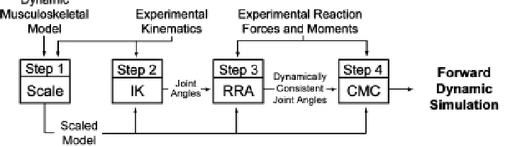
(Delp et al., 2007). OpenSim uses a four-step process to perform dynamic simulation of
experimentally recorded x-y-z marker trajectory data (Figure 8) (Delp et al., 2007); in this
work we focus on the first 2 modeling steps (i.e. scaling and inverse kinematics).
Specifically, in this study we adopted a three-dimensional computational model of the upper
extremity (Holzbaur et al., 2005; Saul et al., 2015) to investigate and identify the movement
characteristics of older adults and compare them with that of young adults (Figure 9).
Figure 9. Computational Model of the Upper Extremity.
Lateral view of model at 45° flexion (A); anterior view of model at 45° abduction (B); anteriormedial view of model (C); posteriolateral view (D). Muscle paths and wrapping surfaces (blue ellipses) are shown (Holzbaur et al., 2005).
The three-dimensional computational model contains three degrees of freedom (DOFs)
at the shoulder including elevation plane, thoracohumeral angle (elevation angle), and
shoulder rotation; two DOFs at the elbow (elbow flexion and forearm rotation); and two
DOFs at the wrist (wrist flexion and deviation) as defined by the International Society of
Biomechanics (Wu et al., 2005). The overall motion of the shoulder joint in this model is
defined by the motions of the clavicle, scapula, and humerus using spherical coordinates
while employing the shoulder motion equations described by de Groot and Brand (2001) to
describe the coupled rotations of the clavicle and scapula. Figure 10 illustrates the degrees of
Figure 10. Computation Model Degrees of Freedom and Axis Definition.
Three degrees of freedom at the shoulder are shoulder elevation (i.e. thoracohumeral angle), shoulder rotation (i.e. rotation about the long axis of the humerus) and elevation plane (0° is in the coronal plane and 90° is anterior in the sagittal plane). In the neutral position, x-axis is anterior/posterior; y-axis is superior/inferior; z-axis is medial/lateral (adapted from Vidt, 2014).
We use scaling and inverse kinematics to fit the musculoskeletal model to the
experimentally-measured kinematic trajectories and to solve for joint angles during measured
movements. In the first step, the musculoskeletal model is scaled to accurately match the
anthropometry of an individual subject. The dimensions and inertial properties of each body
segment in the model are scaled based on a least squares minimization of the locations of the
anatomical markers obtained from motion capture and the virtual markers affixed to the same
anatomical locations in the model. To solve the inverse kinematics problem, the model
generalized coordinate values (in this case, shoulder, elbow, and wrist rotations) which best
produce the raw motion-capture data are calculated as an optimization problem which
minimizes the differences between the experimental marker data and the simulated virtual
maker locations under specific joint constraints such as shoulder angle range of motion
(Figure 11). Specifically, the optimization problem is to minimize the weighted least squared
𝑠𝑞𝑢𝑎𝑟𝑒𝑑 𝑒𝑟𝑟𝑜𝑟 = ∑ 𝑤𝑖(𝑥⃑𝑖 𝑠𝑢𝑏𝑗𝑒𝑐𝑡
− 𝑥⃑𝑖𝑚𝑜𝑑𝑒𝑙) 2 𝑚𝑎𝑟𝑘𝑒𝑟𝑠
𝑗=1 + ∑ 𝑤𝑗(𝜃⃑𝑗
𝑠𝑢𝑏𝑗𝑒𝑐𝑡
− 𝜃⃑𝑗𝑚𝑜𝑑𝑒𝑙) 2 𝑗𝑜𝑖𝑛𝑡 𝑎𝑛𝑔𝑙𝑒𝑠
𝑖=1 (1)
where 𝑥⃑𝑖𝑠𝑢𝑏𝑗𝑒𝑐𝑡 and 𝑥⃑𝑖𝑚𝑜𝑑𝑒𝑙 are the marker locations for the subject and model respectively;
𝜃⃑𝑗𝑠𝑢𝑏𝑗𝑒𝑐𝑡 and 𝜃⃑𝑗𝑚𝑜𝑑𝑒𝑙 are the joint angles for the subject and model respectively; and 𝑤𝑖 and
𝑤𝑗 are weighting factors that allow markers and joint angles to be weighted differently.
Figure 11. Inverse Kinematics in OpenSim.
Blue markers indicate experimental marker locations; pink markers indicate virtual marker locations.
1.2.2 Structure of Thesis
This thesis evaluates age-related differences in kinematic strategies for the performance
of upper limb reaching tasks with varying postural and load demands. To improve
interpretation of these time-series data structures, without underutilizing the large pool of
data, this work employs advanced statistical methods. Thus this thesis will comprise the
following chapters:
This chapter provides the context and background for the development of the SPM method,
its extension to biomechanical applications, and the formulation necessary to conduct the two
sample t-tests used in the analyses of age-related effects on kinematics.
Chapter 3: Age-Related Differences in Kinematics as Influenced by Load and Postural
Demands (Coauthors: Katherine Saul, PhD; Anthony Santago; Meghan Vidt, PhD)
This chapter describes an experimental exploration of the effect of load and postural
demands on age-related kinematic changes, with analyses employing both discrete and SPM
analyses methods.
Chapter 4: Conclusions and Future Work
This chapter provides perspective on the findings and conclusions drawn from Chapter 3, and
CHAPTER 2: STATISTICAL PARAMETRIC MAPPING
The use of advanced statistical methods in the field of biomechanics has become more
necessary, as a variety of biomechanics data, such as motion capture and electromyography
(EMG), can be recorded fairly easily. However, with the increasing level of data collection
capability, a need for more sophisticated statistical analysis methods becomes important.
Biomechanics data often includes continuous time-series data that describe the trajectories of
an entire movement. These time-series data can be seconds or minutes in length. To use
conventional discrete statistical methods, such as t-tests and ANOVA, continuous data is
frequently dissected into single metrics such as peak or mean representative values (Ketcham
et al., 2002; Hortobágyi et al., 2003; Darling et al., 1988) or range of motion (Hortobágyi et
al., 2003). As a result, a significant portion of the data is lost while eliminating the possibility
of conducting analyses on the entire movement pattern. Additionally, the data collection
efforts are substantially devalued. Another disadvantage related to using traditional discrete
statistical methods to analyze extracted single values is that once these discrete values are
extracted from the time-series data, the investigator loses the direct representation of the data
in its original time-series axes, making it more difficult to interpret.
As these limitations are discovered, an increasing number of attempts have been made
to retain the continuous characteristics of biomechanics data and fully investigate the entire
movement trajectory. These attempts include statistical parametric mapping (SPM) (Pataky,
2010; 2012; Pataky et al., 2013) and functional data analyses (FDA) (Ramsay and Silverman,
2002; 2005). In general, these methods represent the continuous time-series data as a
overall significance. In this thesis, our focus is on the use of SPM for biomechanical
statistical analyses.
2.1 Background of SPM and Developments
2.1.1 SPM introduction
Statistical Parametric Mapping is a structure of analysis methods initially developed in
the field of neuroscience (Friston, 2004; Friston et al., 2007) to assess spatially extended
statistical processes used to test hypotheses posed on functional imaging data. SPM can be
used to analyze imaging data including fMRI, PET, and EEG (Friston et al., 2007). SPM has
been used to identify differences in brain activity recorded during functional neuroimaging
experiments. Brain imaging data are represented as voxel maps that are correlated both
spatially and temporally. Brian activity linked to a specific function will change with
different experimental stimulus and can be identified as responsible for that neurological
process. SPM is a voxel-based approach that can identify areas in the brain that are
coactivated under a certain stimulus due to increased perfusion and neural pool activities.
This coactivation pattern is based on the theory that neurons in certain cortical areas have
common responsiveness, so given a definitive stimuli, changes that happen in the brain
should only be found in the area of interest and not elsewhere (Friston, 2004).
Neuroscientists chose SPM to handle large data sets (i.e. voxel maps) with high spatial and
temporal correlations, disregard random effects (e.g. noise in imaging processing) that are
irrelevant to the brain function, and only consider statistically significant differences in
activity changes. Similarly, biomechanical data can be analyzed more accurately using SPM
In general, the analysis process for neuroimaging data requires the data be realigned,
spatially normalized, and smoothed so that a brain structure or area conforms to a known
anatomical space (Friston, 2004; Friston et al., 2007) (Figure 12). This is analogous to
normalization of biomechanics data in which subjects’ time-series data are normalized to the
percentage of movement for equivalent comparisons between or within subjects. Statistical
analysis is then carried out through the use of general linear model (GLM) to estimate
parameters that could explain the patterns shown in the data. This is analogous to the use of
GLM or any of its simplified versions (e.g. t-tests, f-tests, and linear regression) in traditional
univariate statistical analyses. SPM is a mass-univariate approach which considered the
entire dataset in a single analysis, which can be visualized as an SPM image with statistic
values for each spatial or temporal location (Friston, 2004). With this image, SPM then
employs classical inference to determine whether a significant difference exists at a given
location, using Gaussian Fields to identify responses to various experimental factors.
Gaussian random field theory (RFT) is used to describe the probabilistic behaviors of the
SPM maps, as well as resolving multiple comparison problems that could arise during the
statistical inference processes. As a result, the RFT outputs a corrected p value for the
continuous time-series data. This is analogous to the Bonferroni corrections made to correct
for multiple comparison problems in discrete data analysis (Friston, 2004). Biomechanical
data that contain physiologically-correlated data points can benefit from this analysis
approach using GLM and RFT to consider data covariance. In the context of this thesis, we
implementing two sample t-tests in SPM for the analyses of kinematic differences between
young and older adults.
Figure 12. General Procedures to Implement SPM.
Realignment removes movement or shape-related differences to conform the data to the required anatomical space based on a moving average autoregression model. This alignment is necessary to remove differences between subjects or due to scan variances from a single subject; Spatial normalization ensures all subjects’ brain images conform to some standard anatomical space; Spatial smoothing increases the signal-to-noise ratio while convolving with a Gaussian kernel for later uses; Statistical analysis uses the general linear model (GLM) to analyze specific effects observed in the brain; Statistical inference uses Gaussian random field theory to interpret whether effects are significant (corrects the p value) after taking into account non-independent comparisons (correlated factors) (Friston, 2004).
2.1.2 The General Linear Model
The general linear model (GLM) can be formulated to conduct two sample t-tests in the
comparisons of group means. In this study, we develop the two sample t-tests in GLM form
functional tasks. Generally, statistical models are used to describe the relationship between
the variables which affect the experimental outcomes. By using a good model, we are able to
identify the experimental factors that are important in producing the outcomes of the tests.
GLM is a powerful tool in modeling experimental outcomes and most analyses are simply a
variation of it. The general linear model is formulated as:
𝒀𝒏 = 𝑿𝒏𝒎𝜷𝒎+ 𝜺𝒏 (2)
where 𝒀𝒏 (n= 1,2,…N) is a vector representing the experimental outcomes, namely the response variables; 𝑿𝒏𝒎 (m = 1,2,…M) is the design matrix representing explanatory variables that are significant in the experimental design (e.g. age, race, or can be dummy
variables that indicate the level of an experimental factor); 𝜷𝒎is a vector representing the
contribution of each explanatory variable; and 𝜺𝒏 is a vector representing independently, identically, and normally distributed error terms (Kiebel and Holmes, 2004). It should be
noted that each column of the design matrix represents one explanatory variable (also known
as regressors or covariates).
Equation (2) written in matrix form is simply a set of linear equations. To understand
how well this fitted model fits the actual data, the slopes and intercepts of the linear
equations need to be calculated. However, because the number of parameters M is typically
less than the number of response variables N, this set of linear equations cannot be solved.
Thus, estimations of the parameters are made based on the principals of the residues of
sum-of-squares which represents the sum of square differences between the actual and fitted
𝜷̂ = (𝑿𝑻𝑿)−1𝑿𝑻𝒀 (3)
𝑿 and 𝒀 in Equation (3) are the design matrix and the experimental outcomes, respectively.
In the context of two-sample t-test represented in the GLM form, the following expression is
derived under the null hypothesis that the means of the joint angles of young and older adults
(𝜇1, 𝜇2, respectively) are equal to each other, specifically 𝜇1 = 𝜇2:
𝑌𝑞𝑛 = 𝑥𝑞𝑛1𝛽1+ 𝑥𝑞𝑛2𝛽2+ 𝜀𝑞𝑛 (4)
where n indicates the number of data points in either group; q is the group indices (q=1,2);
𝑥𝑞𝑛1 is a dummy variable that equals to 1 when q=1 and 0 otherwise (i.e. q=2) for an
observation in the first group, while 𝑥𝑞𝑛2 is another dummy variable which equals to 0 when
q=1 and 0 otherwise for an observation from the second group (Kiebel and Holmes, 2004).
Consequently, the design matrix in comparing the means of the young and older adult data is
composed of 2 columns of dummy variables (ones and zeros) indicating group membership
and 𝜷 = [𝜇1, 𝜇2]𝑇(Kiebel and Holmes, 2004). In matrix form, Equation (4) can be rewritten
as the following by assuming 𝑛1 measurements in the first group and 𝑛2 measurements in the second group:
𝒀 =
( 𝑌1
⋮ 𝑌𝑛1
𝑌2 ⋮ 𝑌𝑛2)
= ( 1 0 ⋮ ⋮ 1 0 ⋮ 0 0 1 ⋮ 1)
(𝜇𝜇1
2) +
( 𝜀1
⋮ 𝜀𝑛1
𝜀2 ⋮ 𝜀𝑛2)
(5)
It should be noted here 𝑌1… 𝑌𝑛1represents from the first to the last observation taken in the
first group; 𝑌2… 𝑌𝑛2represents from the first to the last observation taken in the second group.
can be modeled as a matrix containing multiple data points per observation (i.e. each
measurement taken as time-sequence continuum). This is how the entire movement trajectory
of each observation (e.g. subject) can be modeled as a function rather than being extracted as
individual data points in time. To compare group means with a two sample t-test and
determine whether age has an effect on mean kinematic trajectories, we are testing the null
hypothesis 𝒄𝑻𝜷 = 0 where 𝒄 = [1, −1]𝑇 to achieve equal means between the two groups (Kiebel and Holmes, 2004). The specific t statistic is computed from:
𝑻 = 𝒄𝑻𝜷̂
√𝝈̂𝟐𝒄𝑻(𝑿𝑻𝑿)−𝟏𝒄 (6)
where 𝝈̂𝟐 is the residual variance estimated by the residues of sum-of-squares divided by the degrees of freedom (Kiebel and Holmes, 2004). With 𝑛1and 𝑛2 measurements in each group,
we have: (𝑿𝑻𝑿) = (𝑛1 0
0 𝑛2) → (𝑿𝑻𝑿)−𝟏 = (
1/𝑛1 0/𝑛1
0/𝑛2 1/𝑛2) → 𝒄
𝑻(𝑿𝑻𝑿)−𝟏𝒄 = 1 𝑛1+
1 𝑛2,
resulting in the t statistic:
𝑇 = 𝜇̂1−𝜇̂2
√𝜎̂2(1/𝑛
1+1/𝑛2)
(7)
Equation (7) is the same formulation as the standard two sample t-tests with 𝑛1+𝑛2-2 degrees of freedom under the null hypothesis 𝜇1 = 𝜇2 (Kiebel and Holmes, 2004). In this manner, joint angle trajectories can be compared between young and older adults in this study.
2.1.3 Statistical Inference
Following the development of a model of the experimental outcomes, we must infer
whether there is a difference between the group means or make judgments on the probability
above purposes and makes comments about specific responses to experimental factors
(Friston, 2004). A common concern in making inferences is the issue of making multiple
comparisons simultaneously. For example, the data we have collected in movement analysis
often have multiple spatial as well as temporal dimensions. Consequently, to determine if this
search volume (e.g. the brain volume, group x subjects x time-series data) shows any
evidence of an effect, we are challenged with multiple comparison problems that involve
hundreds and thousands of statistical values. Therefore, it is crucial to take the correlation
between data points into account when making inference and make corrections to the
corresponding p values before drawing conclusions regarding the significance of the data.
2.1.4 The Multiple Comparison Problem and Family Wise Error Rate
To handle the multiple comparison problem, it is important to realize we often have no
information on where in the dataset significant differences may be observed. Therefore the
null hypothesis should be made over the total search volume, which results in a family of
statistics. The risk of error associated with these statistics is called the Family Wise Error rate
(FWE) and it describes the probability that a family of data values could have arisen by
chance. One method to test this family wise null hypothesis is called “height thresholding”,
in which a threshold is applied to each statistical value such that any value above that
threshold is not likely to have been observed by chance. Consequently, significant difference
is concluded at the location(s) where statistical value(s) are found to be above that threshold
(Brett, Penny and Keibel, 2004). In traditional statistical analyses, the threshold value is also
One of the simplest and most conservative method used to handle the multiple
comparison problem is the Bonferroni correction. The basic principle behind the Bonferroni
correction is that in order to avoid a large number of false positives, the alpha threshold must
be lowered to take the multiple number of comparisons into account. Given a selected
threshold value 𝛼 for each of the n number of tests, the probability that all n tests will be less than 𝛼 is (1 − 𝛼)𝑛. Therefore, the family wise error rate 𝑃𝐹𝑊𝐸 is then 1 − (1 − 𝛼)𝑛 ,
indicating the probability that one or more values will be greater than 𝛼. This expression can be simplified additionally to the following form (Brett, Penny and Keibel, 2004):
𝑃𝐹𝑊𝐸 ≤ 𝑛𝛼 (8)
By approximation and solving for 𝛼, we can see that the Bonferroni correction method assigns a threshold value of 𝛼 of 𝑃𝐹𝑊𝐸/𝑛 to each test. It is important to see here that this threshold will be significantly reduced with an increasing number of comparisons. For
example, if we set the threshold at 0.05 (i.e. 𝑃𝐹𝑊𝐸 = 0.05), with 1000 tests, the corresponding
𝛼 value is then 0.00005. This significantly reduces the likelihood for the individual p values
to reach significance (i.e. the null hypothesis becomes much more difficult to reject). Thus,
the Bonferroni correction is considered conservative. Furthermore, since the Bonferroni
correction method makes corrections on a collection of discrete values, the correlations
between neighboring values are ignored; in fact, if values covary, then there are much fewer
independent tests than assumed. The correlation between neighboring values arises from the
nature of physiological data, and the number of correlated data points are also increased with
large amount of post-processed, smoothed data, it is more difficult to determine the number
of independent tests involved in this multi-dimensional data space.
2.1.5 Random Field Theory
An alternative approach to address the multiple comparison problem is based on the
theory of random fields, or Random Field Theory (RFT). RFT is used in SPM to identify
regionally-specific effects in smooth statistical maps, detecting whether there is an effect in
the region of interest while handling the multiple comparison problem (Worsley, 2004).
Explicitly, RFT finds the height threshold for the statistical map with a given family wise
error rate (Brett, Penny and Keibel, 2004). The concept is that threshold values can be
adjusted while accounting for the fact that the neighboring data points are not independent by
virtue of continuity in the original data and that the values in a random field are spatially
correlated (Friston, 2004).
RFT solves the multiple comparison problem by using the results obtained from the
parameter called the expected Euler characteristic (EC). The expected EC value is interpreted
as the number of clusters above a desired threshold. We are interested in the data above the
desired threshold because to reject the null hypothesis, the resulting p value needs to be
smaller than the 𝑃𝐹𝑊𝐸 value (i.e. 0.05) which indicates a larger t (or Z) value. It should be noted that the RFT is based on result of smoothed statistical maps, therefore the smoothness
of the (i.e. the correlation) of the data need to be calculated. Specifically, the full width half
maximum (FWHM) smoothing kernel was applied in the implementation of RFT and this
value can be used to calculate the parameter ‘Resels’, or resolution elements. Brett, Penny
the same size as the FWHM and is similar to the number of independent observations. At
high thresholds, the expected EC value denoted by Ε(𝐸𝐶) approximates the FWE rate
(𝑃𝐹𝑊𝐸 ≈ Ε(𝐸𝐶)). In the two-dimensional data spectrum case (e.g. joint angle as a function of
time), Ε(𝐸𝐶) can be calculated based on Equation (9). Consequently, with a desired 𝑃𝐹𝑊𝐸 at 0.05, the Z score threshold 𝑍𝑡 can be calculated to set the threshold and determine how many clusters of values are above this threshold.
Ε(𝐸𝐶) = 𝑅(4𝑙𝑜𝑔𝑒2)(2𝜋)− 3
2𝑍𝑡𝑒−
1 2𝑍𝑡
2
(9)
RFT declares significance over a connected volume or region of the SPM, which
includes all the data points that make up the volume. In this manner, RFT is also much more
sensitive to significance. The exact number of data points in the experimental outcomes is
actually irrelevant because RFT expresses the search volume in terms of smoothness or
Resels. Once any connected volume or region of SPM exceeds a predetermined threshold
value, we conclude that significance is observed. Figure 13 shows an example of an image
thresholded at two difference levels. In this thesis, the methods used in RFT described here
can reveal an entire movement interval where significant kinematic differences between
groups may occurs rather than discrete peaks or valleys. This is very important because
intuitively, one may expect statistically significant differences in a movement to occur over a
Figure 13. Random Field Theory Applied at Different Thresholds.
a. A three dimensional plot with no applied threshold; b. thresholded plot at Z = 0; c.
Thresholded plot at Z = 1; d, e. Top view of observed thresholds. The thresholded values are randomly chosen for illustration purposes. (adapted from Lea Firmin and Anna Jafarpour lecture, 2009)
2.2 Application of SPM in Aging Movement Change Evaluations
2.2.1 General Statistical Methods in Biomechanics
Discrete statistical analysis methods used to analyze movement data can underutilize
large datasets describing movement, as well as introduce bias. Pataky et al. (2013) have
discussed various sources of bias related to traditional statistical approaches in biomechanics.
First, the so-called “directed” hypothesis may introduce bias by considering only a limited time
window of the movement, while absolute maximum or minimum values may be found in other
areas outside the predetermined region; this results in post hoc regional focus bias (Pataky et
al., 2013). Second, bias may arise from the “non-directed” hypothesis in which
physiologically-related components (such as the degrees of freedom of a limb) are examined
Therefore ignoring covariance factors may result in the inter-component covariance bias
(Pataky et al., 2013).
SPM eliminates regional focus bias and allows hypotheses to be proposed over the entire
spectrum. SPM also addresses the multiple comparison problem and therefore eliminates the
covariance bias. In addition, using the methods in SPM allows the results to be presented in
their original spatiotemporal biomechanical data spectra, resulting in a more intuitive
understanding regarding the context for regions for which significant differences are detected
during movement. Furthermore, since SPM provides maps of the calculated statistical values,
results or significance over the entire movement trajectory or a small portion of the movement
can be identified immediately. Therefore, meaningful conclusions may be drawn over that
portion of the movement.
2.2.2 Prior application of SPM to biomechanical data
Several prior studies have demonstrated uses of SPM in biomechanics (Pataky, 2010;
2012; Pataky et al., 2013), and compared SPM analyses to discrete analyses. Example
applications have included analyses of walking speeds on 1D vertical ground reaction force
during stance phase (Figure 14a, c), 2D peak foot pressure (Figure 14b, d left), and 3D
spatiotemporal pressures (Figure 14b, d right); as well as probing probabilistic simulations of
biomechanical data (Pataky, 2010). These applications demonstrate the effectiveness of SPM
Figure 14. Applications of SPM in Biomechanical Analyses.
a. 1D vertical ground reaction force (vertical GRF) time series during three walking speeds; b. 2D mean peak pressure image during three walking speeds (left), 3D pressure image time series during three walking speeds (right); c. 1D SPM results of vertical GRF time series, shaded grey area indicate significance effect of walking speed on vertical GRF; d. 2D SPM results of mean foot pressure; colored regions represent significant effect of walking speed on peak pressures (left). 3D SPM results of foot pressure; colored regions represent
significant effect of walking speed on spatiotemporal foot pressures (right) (Pataky, 2010).
SPM has been compared to discrete methods for a broad range of biomechanical data
including ground reaction forces (GRFs) (Pataky, 2010), kinematics (Pataky et al., 2013),
and muscle forces (Pataky et al., 2013). In the investigation of the effects of walking speed
on GRFs, SPM revealed correlation between the two over almost the entire stance phase as
compared to a single p value in the discrete case (Figure 14 a, c). Positive or negative
correlations can be concluded directly from the SPM{t} map as well (i.e. values above the
zero line in the SPM{t} map indicate positive correlation; values below the zero line in the
SPM{t} map indicate negative correlation). In the study of kinematic data, SPM once again
identified which vector component was the main contributor to the observed significant
differences.
In general, the outcomes of SPM were consistent with the results of discrete
(traditional) statistical methods qualitatively. However, in some cases these two approaches
can yield different results. Pataky (2013) attributed these discrepancies to the bias inherent in
discrete analysis: regional focus bias (i.e. directed hypotheses) and inter-component
covariance bias from ignoring covariance factors (i.e. non-directed hypotheses). Furthermore,
when extreme values are extracted from the time series data (in discrete analyses), other
effects present in the data are ignored. In this case, it is possible that SPM will result in
statistical conclusions that differ from discrete methods because it is highly likely that at least
one point extracted from the original dataset (in discrete analyses) will exceed the
uncorrected threshold simply by chance (Pataky et al., 2013). Pataky also recognized other
sources of bias that can be present in the applications of SPM such as unit normalization.
However, these additional sources are not unique to SPM.
To explore the applications of SPM, many open source software packages are available
for the analyses of imaging and biomechanical data. These packages include SPM1D
(http://www.spm1d.org/index.html), SPM12 (http://www.fil.ion.ucl.ac.uk/spm/software/),
and fMRIstat (http://www.math.mcgill.ca/keith/fmristat/). Specifically, SPM1D is designed
for one dimensional SPM analysis in Python (Python Software Foundation, DE) and Matlab
(The Mathworks, Natick, MA) to demonstrate a variety of uses in biomechanics. SPM12 and
CHAPTER 3: AGE-RELATED DIFFERENCES IN KINEMATIC STRATEGY AS INFLUENCED BY LOAD AND TARGET LOCATION
3.1 Introduction
Aging is commonly associated with diminished ability to perform activities of daily
living (ADLs) and loss of independence and mobility (Clark and Manini, 2010; Landers et
al., 2001), which directly affects quality of life and can increase the reliance of these
individuals on caregivers. By 2050, nearly 89 million people (or over 20% of the US
population) will be over the age of 65, leading to a 25% increase in health care costs by 2030
(Center for Disease Control and Prevention and Prevention, 2013). Factors contributing to
age-related reductions in function include changes in muscle architecture and changes in
movement patterns. Reductions in muscle mass (i.e. sarcopenia) and muscle quality are
typical (Clark and Manini, 2010; Sayer et al. 2008; McDonagh et al., 1984; Morley, 2012;
Narici and Maffulli, 2010; Rosenberg, 1997). Approximately 5% of older adults aged 65
experience sarcopenia, and this prevalence increases to 50% in people 80 years and older,
which leads to reduced muscle strength and power (dynapenia) (Hughes et al., 2001; Morley,
2012). Other factors such as declines in muscle pennation angle and altered motor unit firing
patterns can also contribute to the loss of strength (Janssen, 2010; Morley, 2012).
These changes in muscle architecture may underpin observed changes in movement
patterns with age (Kozak et al., 2003; Lu et al., 2006; Morgan et al., 1994; Tsai and Lin,
2015). In particular, increased stability demands have been reported in older cohorts. Older
adults had more problems maintaining stability during quiet standing when compared to