Results on point and interval estimation for log linear models with non ignorable non response

Results on point and interval estimation for log-linear models with

non-ignorable non-response

Paul S. Clarke and Peter W. F. Smith

Abstract

It is common that log-linear models for multi-way contingency tables with one variable

subject to non-ignorable non-response will yield non-response boundary solutions, where the

probability of non-respondents being classified in certain cells of the table is estimated to be

zero, resulting in infinite estimates for some of the log-linear parameters. This paper

investigates the effect of such non-standard behaviour on the maximum likelihood estimator.

Provided that the model parameters are identifiable from infinite samples, it is demonstrated

that: 1) existence and uniqueness of the maximum likelihood estimates is assured under weak

conditions; and 2) the maximum likelihood estimator is consistent and asymptotically normal.

However, boundary solutions do result in a singular information matrix, which prevents

calculating confidence intervals based on a normal approximation to the maximum likelihood

estimator; it is shown that these singularities can be removed by a simple transformation of

the log-linear parameters.

Paul S. Clarke

Department of Infectious Disease Epidemiology, Imperial College London, St. Mary’s Campus, Norfolk Place, London W2 1PG, U.K.

Peter W.F. Smith

Southampton Statistical Sciences Research Institute, University of Southampton, Highfield, Southampton SO17 1BJ, U.K.

Abstract:

It is common that log-linear models for multi-way contingency tables with one variable subject to ignorable response will yield response boundary solutions, where the probability of non-respondents being classified in certain cells of the table is estimated to be zero, resulting in infinite estimates for some of the log-linear parameters. This paper investigates the effect of such non-standard behaviour on the maximum likelihood estimator. Provided that the model parameters are identifiable from infinite samples, it is demonstrated that: 1) existence and uniqueness of the maximum likelihood estimates is assured under weak conditions; and 2) the maximum likelihood estimator is consistent and asymptotically normal. However, boundary solutions do result in a singular information matrix, which prevents calculating confidence intervals based on a normal approximation to the maximum likelihood estimator; it is shown that these singularities can be removed by a simple transformation of the log-linear parameters.

1 Introduction

Consider a multi-way contingency table cross-classified by k variables, X1,…, Xk, each with nominal categorical outcomes. If Y = Xk is subject to non-response then the observed data are incompletely classified. Baker and Laird (1988) introduced a family of log-linear models for incomplete tables of this type, which have been considered by other authors (Baker et al. 1992; Park and Brown 1994; Clarke 1998; Forster and Smith 1998; Park 1998; Smith et al. 1999; Clarke 2002; Clarke and Smith 2004). Such ‘Baker and Laird’ models are important because they permit estimation of the coefficients in the regression of Y on X1,…, Xk−1 under non-ignorable non-response. In Baker and

Laird models, non-response is ignorable if the probability of missing Y is independent of Y given

X1,…, Xk−1; hence, it follows that non-response is non-ignorable if the probability of Y being missing

depends on Y itself, even after controlling for X1,…, Xk−1. (The conditions required for valid inference

under ignorable non-response are delineated by Rubin (1976).)

Baker and Laird models can produce extreme and implausible point estimates called response boundary solutions. A response boundary solution occurs when the probability of respondents being classified in certain cells of the table is estimated to be zero. For example, non-ignorable models were used by Smith et al. (1999) to estimate the proportion voting for each party in a pre-election survey where voting intention was missing for a subset of sampled individuals; the maximum likelihood (ML) estimate of the proportion of non-respondents intending to vote for the Labour Party was estimated to be zero, despite the model fitting the data well. A simulation study by Clarke (1998) showed that the probability of a boundary solution could be zero and non-negligible in finite samples, even when the Baker and Laird model is the true population model.

A consequence of such non-standard behaviour is that point estimates of certain log-linear parameters can be ±∞. Infinite estimates can also occur when fitting log-linear models to completely classified but sparse contingency tables; that is, observed tables with one or more cells having frequency zero. Difficulties on determining the existence, uniqueness and calculation of ML estimates for sparse tables were resolved by developing a theory of ‘extended’ ML estimation (Haberman 1974, Wedderburn 1976, Clarkson and Jennrich 1991). In this paper, these issues are considered for response boundary solutions in a simple ignorable Baker and Laird model. The findings for non-response boundary solutions and sparse contingency tables are compared in the discussion.

information matrix becomes singular. In the last part of this paper, it is demonstrated why an exponential transformation obviates this problem.

2 Preliminaries

2.1 Notation

Recall that X1,…, Xk−1 and Y are nominal categorical variables and that Y is incompletely observed.

Let Y have levels numbered from 1 to q, and let Xj have levels numbered 1 to sj (j = 1,…, k − 1) with s = ∏jsj. Further define the response indicator variable as R, equal to 1 if Y is observed and 2 otherwise. The resulting (k + 1)-way contingency table of X1,…, Xk−1, Y and R is referred to as the complete data

table; that is, the hypothetical multi-way table which would have been be observed if the missing outcomes of Y were known. Denote the cell frequencies of the complete data table by the column vector z = {zxyr}, where zxyr is the (possibly unknown) sample frequency classified by X = x, Y = y and

R = r; X = (X1,…, Xk−1)T and x = (x1, …, xk−1)T. It is assumed that z is a realisation of the multinomial

random vector Z = {Zxyr} ~ MN(n, π), where n = z+++ and π = {πxyr} are the cell frequencies.

2.2 Model specification

In general, Baker and Laird models are selection models defined by two sub-models called the ‘margin’ model and the ‘non-response’ model. The margin model is log-linear for the joint distribution of X and Y. For k = 2 the margin model is defined as

log(πxy+) = ν + λX(x) + λY(y) + λXY(x, y), (1)

where X = X1, corner-point constraints fix λX(1) = λY(1) = λXY(1, y) = λXY(x, 1) = 0 for all x, y without

loss of generality, and ν is the normalising constant ensuring ∑x,yπxy+ = 1. The interest parameters are

the sq non-zero log-linear parameters of the margin model. The non-response model is a logistic regression of R on X and Y, which specifies how Y came to be missing or observed. Returning again to the k = 2 example, the regression model can be written

log(π2|xy / π1|xy) = λR(2) + λXR(x, 2) + λYR(y, 2) + λXYR(x, y, 2), (2)

the same corner-point constraints as the interest parameters. Together, (1) and (2) define the cell probabilities for the complete table as πxyr = πxy+πr|xy. Generalising (1) and (2) to k > 2 is straightforward.

The focus of this paper is on the case where the probability of non-response depends only on Y

and the margin model is saturated; that is, all interactions between X and Y are included in the margin model. For notational simplicity, the multivariate X is replaced by the single covariate, X, each level of which corresponds to one of the s cross-classifications of X. Using this notation, if non-response depends only on Y, this model is defined by (1) and (2) under the further constraints that λXR_{(x, 2) =}

λXYR_{(x, y, 2) = 0 for all x, y.}

It was shown by Baker and Laird (1988) that, when λXR_{(x, 2) = λ}XYR_{(x, y, 2) = 0, inferences} based on the log-linear model

log(πxyr) = ν + λX(x) + λY(y) + λR(r) + λXY(x, y) + λYR(y, r) (3)

are equivalent to (1) and (2), where ν now ensures that ∑x,y,rπxyr = 1 and corner-point constraints are used as before. This result holds in general provided that the margin model is saturated. Model (3) is an important special case that has been the focus of previous work. The primary reason for this is that (3) is the most parsimonious non-ignorable model allowing estimation of the unrestricted cell probabilities of the marginal table. The number of free parameters in model (3) is p = q(s +1)– 1, the sum of the non-zero parameters in the margin and non-response models less one (ν is a function of the remaining non-zero parameters). Denote the p free log-linear parameters of model (3) by the vector λ = {λX_{(2),…, λ}YR_{(q, 2)}}T _{with corresponding parameter space Λ=ℜ}p_.

2.3 Maximum likelihood estimation

For cases where R = 2, Y is missing and so z is incompletely observed. Only the cells of the observed data table zobs = (z111,…, zsq1, z1+2,…, zs+2)T are known, which are outcomes from random vector Zobs. It

follows that the log-likelihood for λ is (ignoring the additive constant)

l(λ; zobs) = ∑x,yzxy1log(πxy1) + ∑xzx+2log(∑yπxy2), (4)

where π is defined by (3) (c.f. Baker and Laird 1988). Throughout this paper, λˆ =

T

)} 2 , ( ˆ , ), 2 ( ˆ

{λX _KλYR q will be used to denote the ML estimate minimising (4), and also the ML estimator of λ, depending on the context. Under multinomial sampling, the observed data have s(q +

1) − 1 degrees of freedom. Hence, it is necessary for identifiability that p ≤ s(q + 1) − 1, which

henceforth be assumed that the complete data are realisations from model (3) with true parameter λ ∈ Λ and sample size n.

2.4 Non-response boundary solutions

Definition 1: A non-response boundary solution for model (3) is a ML estimate such that

π

ˆ_xy2 = 0 for

at least one combination of xand y (Baker and Laird 1988).

In terms of the log-linear parameters, a non-response boundary solution for model (3) implies that

) 2 , ( ˆ ) 2 (

ˆR _λYR _y

λ + = –∞, and hence that πˆ+y2 = 0. If the non-response boundary solution is such that 1

∉ {y :πˆ_+y2 = 0} and

π

ˆ_xy1 > 0, then this implies that _λˆYR(y,2)=−∞ _because

1 ˆ_xy

π

> 0 implies

_λ

ˆR(2)

∈ ℜ. However, if 1 ∈ {y :πˆ_+y2 = 0} and

π

ˆ_xy1 > 0 then _λˆR(2)_+λˆYR(y,2) _{∈ ℜ, but}

_λ

ˆR_{(2)=−∞ and}

+∞ =

) 2 , ( ˆYR _y

λ

. In other words, neither

_λ

ˆR(2) _nor

_λ

ˆYR_{(y,2) is finite, but their sum is; this is an} artefact of the corner-point constraints used to identify the log-linear parameters and so not of interest in this paper. Hence, only non-response boundary solutions where 1 ∉ {y :πˆ_+y2 = 0} will be

considered in this paper; this is done without loss of generality because the levels of Y are nominal and

so can be recoded, changing a

π

ˆ₊₁₂ = 0 solution to an equivalent one where

π

ˆ₊₁₂ ≠ 0.

3 Alternative Model Parameterisation

Under model (3), the cell probabilities can be factorised as

πxyr = αrβy|rγx|y, (5)

where αr = Pr(R = r; λ), βy|r = Pr(Y = yR = r; λ) and γxy = Pr(X = xY = y; λ), for all x, y and r.

Then, using this parameterisation, the log-likelihood function can be re-written as

l(α, β, γ; zobs) =

∑

+

∑

₊

∑

y

x x y

y x y x

y x y

xy z

z

,

| 2 | 2 2

| 1 | 1

1log(αβ γ ) log( α β γ ), (6)

where α = (α1, α2)T, βr = (β1r,…, βqr)T, γy = (γ1y,…, γsy)T, βT = (β1T, β2T), and γT = (γ1T,…, γqT). This function can be split into two additive components, one depending on α and β1, and the other

depending on β2 and γ, which can be maximised separately. Maximising the first component gives αˆr

have a simple analytical expression, although it can be interpreted geometrically. The perfect-fit log-likelihood is obtained by substituting πˆxy1=zxy1/n and πˆx+2 = zx+2 / n into (4). The deviance is twice

the difference between the perfect-fit log-likelihood and (6), and simplifies to

∑ ₊ + ₊₊

=

yz y D( y ,ˆy) 2z D( ,ˆ) 2

) ˆ , ˆ

dev(β₂ γ ₁ p ₁ γ ₂ p₂ µ , (7)

where µ = (µ1,…, µq)T = ∑yγyβy|2, µx = ∑yγx|yβy|2 = Pr(X = x | R = 2; λ), py1 = (p1y1,…, psy1)T, p2 =

(p12,…, ps2)T, px|y1 = zxy1/z+y1, and px|2 = zx+2/z++2. The function D(a, b) = ∑i ai log(ai / bi) is the Kullback-Leibler distance between a, b ∈ S, where S is the s-dimensional simplex, the space of discrete probability distributions with s mass points. It follows from (7) that the ML estimate is the

point ( T 2 ˆ

β ,_γˆT_{) such that the weighted distance between a) µˆ and p2 and b) each of} y

γˆ and py1, is

minimised. This permits a geometrical interpretation of maximum likelihood estimation, which has been considered graphically by Smith et al. (1999) and Clarke (2002).

4 Results on Maximum Likelihood Esitmation

To investigate the consequences of the ML estimator’s non-standard behaviour, it is first necessary to impose the condition that zobs > 0 (where a > b denotes the condition that every element of vector a is greater than scalar b). Thus the behaviour of non-response boundary solutions can be considered in isolation from those due to sparseness in zobs. Now consider the following lemma.

Lemma 1: Suppose complete data Z follows a multinomial sampling model with the cell probabilities

determined by model (3), and that zobs > 0. Then πˆ_xy1 > 0 and πˆ_x+2 > 0 for all x, y and all λˆ ∈ Λ ∪ bd(Λ).

Proof: Note that, for a given choice of {γˆ }, the space of possible _y µˆ is the convex hull of {γˆ }, _y

denoted by C(γˆ ) ⊆ _y S; the co-ordinates of µˆ in C(γˆ ) - taken with respect to spanning set {_y γˆ } - _y

determine {βˆ_y|2}. Similarly, {py1} is the spanning set for convex hull C(py1) ⊆ S. Hence, the ML

estimate can be visualised as the choice resulting in the vertices of C(γˆ ) and _y C(py1) lying close to

each other, such that the distance between µˆ ∈ C(γˆ ) and _y p2 is minimised. Smith et al. (1999)

- a perfect-fit solution; and (ii) p2 ∉ C(py1) which implies that C(ˆ ) γy ≠ C(py1) such that (7) is

minimised.

In the perfect-fit case (i), then γˆ = _y py1 and µˆ = p2 is the unique solution lying in the interior

of S (zobs > 0 ensures that none of {py1} or p2 lie on the boundary). Therefore, as αˆr = z++r / n > 0

andβˆ_y1| = z+y1 / z++1 > 0, it necessarily follows from (5) that πˆxy1>0 and πˆx+2 =αˆ2µˆx > 0.

For case (ii), it is only required to show that a choice of (βˆT₂,γˆT) can always be made such that |dev(

β

ˆ₂,

γ

ˆ)| < ∞, even if this choice does not necessarily correspond to the minimum deviance

possible. The conditon zobs > 0 ensures that the deviance cannot be −∞; and a choice C(γˆ ) can y

always be found that corresponds to a finite deviance. Hence, whatever the position of p2 relative to

C(py1), no choice of C(γˆ ) exists that both minimises (7) and lies on the boundary of _y S, which implies

that µˆ > 0. This completes the proof.

Note: Clarke and Smith (2004) state that there are between 1 and q − 1 values of y such that

2 ˆ_+y

π = 0 for an arbitrary boundary solution. This can be seen from Lemma 1 because _πˆ_x+2 > 0 implies πˆxy2 > 0 for at least one value of y, which would not be possible if all q values of y were such that πˆ+y2 = 0.

4.1 Existence and uniqueness

If follows from Lemma 1 and (5) that the ML estimate of ‘natural’ parameter ω = (αT_{, β}

1T, γT, µT)T

will be strictly positive provided zobs > 0. This gives us the following result regarding existence.

Result 1: Suppose that {py1} and p2 are distinct points in S and that conditions in Lemma 1 hold.

Then λˆ will always exist and be unique.

Proof: If zobs > 0 then ωˆ > 0 (Lemma 1). Thus a minimum must exist in the interior of the natural parameter space because (7) is continuous, defined almost everywhere, and bounded below by zero

(the perfect-fit solution). Furthermore, given γˆ and µˆ , it is always possible to determine βˆ2 as the

co-ordinate of µˆ ∈ C(γˆ ), provided that _y q ≥ s (which is taken to hold throughout) and {py1} and p2

noting that (7) is convex because it is a weighted sum of convex D(a, b) (for fixed a); uniqueness of λˆ

follows from noting that the mapping from log(πˆ) to is λˆ _one-to-one.

4.2 Consistency

Result 2: Suppose complete data Z follow a multinomial sampling model with the cell probabilities

determined by (3), and that the conditions in Result 1 hold. Then λˆ is consistent for all λ ∈ Λ.

Proof: Consider the random variables Pr = Z++r / n and Py1 = Z+y1 / Z++1. From Section 3, αˆ = r Pr and

1 | ˆ

y

β = Py1, with zobs > 0 ensuring that αˆ , r βˆy1| ∈ (0, 1). The weak law of large numbers (WLLN)

gives that αˆ = r Z++r / n → π++r and Z+y1 / n → π+y1 as n →∞, which implies that αˆ → r αr and (via

Slutsky’s theorem) βˆy|1 = Py|1 = (Z+y1 / n) / (Z++1 / n) → π+y1 π++1=βy|1 in probability.

Now consider the sequence of functions {dev(β2,γ|n,zobs):n=1,2,K} and the corresponding

sequence of ML estimates obtained by maximising each deviance function by {ˆ2,ˆ :n=1,2,K}

n n _γ

β .

Result 1 ensures existence and uniqueness of these estimates. Using the same arguments as above, it

follows that Pxy1 → γxy and Px2 → µx and so _→∞ =

∑

+ + ++

y

y y y obs

n {dev( , |n, )} z D( , ) z D( , )

lim β2 γ z 1 γ γ 2 µµ .

Hence it follows that lim_→∞β =ˆ2 β2

n

n and →∞γ =γ

n n ˆ

lim , which implies β →ˆy|2 βy|2 and γˆy→γˆy in

probability.

Together with Result 1, these results ensure that λˆ → λ as ωˆ → ω, which completes the proof.

4.3 Asymptotic normality

Result 3: Suppose complete data Z follow a multinomial sampling model with the cell probabilities

determined by (3), and that the conditions in Result 1 hold. Then n1/2_(λˆ_{− λ) →}d _{N(0, Γ}−1_{), where Γ is}

the p × p expected single-observation information matrix.

Proof: Asymptotic normality follows from noting that, for large samples, λˆ will lie in a neighbourhood of λ because the estimator is consistent (Result 2). Furthermore, as (4) is a smooth function of λ with finite first, second and third derivatives, and taking expectations with respect to Zobs involves summation over a finite range of discrete values, the conditions given by Cramér (1946, Sec.

and a p × p covariance matrix equal to the inverse of the expected single-observation information matrix.

5 Interval Estimation

It is known from Results 2 and 3 that the ML estimator is consistent and

)

ˆ

(

2 / 1

_{λ −}

_λ

n

→d N(0, Γ−1_{), (8)}

where 0 is a vector of p zeros and Γ is the p × p single-observation information matrix for (4). A general method for calculating Γ−1 _{has been proposed by Oakes (1999) and the performance of these}

intervals has been assessed by Clarke and Smith (2004), where it was noted that Γ is singular for boundary solutions. In this section, the approach of Oakes (1999) is implemented for model (3), and it is demonstrated why Γ is singular for boundary solutions. Details of a simple transformation to remove singularities from Γ` are then given.

5.1 Calculating the expected observed data information matrix.

The score equations for model (3) are obtained by differentiating (4) with respect to the free parameters and setting the resultant system of p equations to zero to give:

0 ˆx₊₊ −zx₊₊ =

nπ for x = 2,…, s, (9a)

0 ˆ₊₊₂−z₊₊₂ =

nπ (9b)

0 ˆ ˆ_{+ +} − _{+ 1}−

∑

₊₂ y_|x =

x x y

y z z

nπ φ y = 2,…, q, (9c)

0 ˆ ˆxy₊ −zxy₁−zx₊₂ y_|x =

nπ φ x = 2,…, s, y = 2,…, q, (9d)

0 ˆ ˆ+ ₂−

∑

+₂ y_|x =

x x

y z

nπ φ , y = 2,…, q, (9e)

where φy|x = Pr(Y = y|X = x, R = 2)

= exp{λY_{(y) + λ}XY_{(x, y) + λ}YR_{(y,2)} / ∑}

y exp{λY(y) + λXY(x, y) + λYR(y,2)}, (10)

for y = 1,…, q.

J, the definition of which is given by Fienberg (1980, p. 170). By differentiating (4) twice with respect to λ and taking expectations with respect to Zobs, it can be shown that

      Ψ − = Γ ηη ησ ση σσ J J J J

, (11)

where Ψ is a singular symmetric matrix, Jσσ, Jση, Jησ and Jηη are sub-matrices of J corresponding to

the partition λT _{= (σ}T_{, η}T_{); σ= {λ}X_{(2),…, λ}X_{(q), λ}R_(2)}T _{and η= {λ}Y_{(2),…, λ}Y_{(q), λ}XY_{(2,2),…, λ}XY_(s,q),

λYR_{(2,2),…, λ}YR_(q,2)}T_{. Similarly, the sub-matrices of the inverse of J are}

      = − ηη ησ ση σσ V V V V

J 1 . (12)

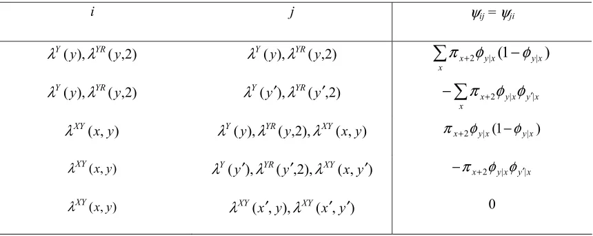
Let ψijbe element (i, j) of Ψ, corresponding to the second derivative of (4) taken with respect to i, j, which are both elements of η, where λT _{= (σ}T_{, η}T_{) is the partition used in (11) and (12). The}

[image:11.612.93.523.395.566.2]

definition of {ψij} is given in Table 1.

Table 1: The elements of Ψ for equation (11).

i j ψij = ψji

) 2 , ( ), (y YR y

Y _λ

λ _λY(y),_λYR(y,2)

∑

−

+

x x yx yx

) 1

( _|

|

2

φ

φ

π

) 2 , ( ), (y YR y

Y _λ

λ _λY(y_′),_λYR(y_′,2)

∑

′ +

−

x x 2 y|x y|x

φ

φ

π

) , (x y

XY

λ _λY(y),_λYR(y,2),_λXY(x,y) _{(1 )}

| |

2 yx yx

x φ φ

π ₊ −

) , (x y

XY

λ _λY(y_′),_λYR(y_′,2),_λXY(x,y_′)

x y x y x+2 | ′|

−π φ φ

) , (x y

XY

λ _λXY(x_′,y),_λXY(x_′,y_′) ₀

Note: Indices are defined for x, x′ = 1,…, s; y, y′ = 1,…, q; x≠ x′; and y≠ y′; and φy|x is defined in (12).

By differentiating the observed data score function with respect to λ and taking expectations

T 1 1       Ψ       + =

Γ− −

ηη ση ηη ση V V L V V

J , (13)

where L = (I – VηηΨ)−1 and I is an identity matrix of the appropriate dimensions. The second term of

the right-hand side can thus be interpreted as the additional variability resulting from the data being incomplete. The derivation of (13) follows from noting that (11) is of the form A − B and (A − B)−1 ₌ A−1 _{+ A}−1_B(I−A−1_B)−1_A−1 _{(Mardia, et al. 1979, A 2.4f). Substituting gives}

T 1 1 1 1 ) ( ) ( 0 0 0       Ψ − Ψ       + =             Ψ − Ψ −       Ψ Ψ +       = Γ − − − − ηη ση ηη ηη ση ηη ησ ση σσ ηη ση ηη ση ηη ησ ση σσ V V V I V V J V V V V V I V I V V V V V V

which simplifies to (13). Calculating (13) requires evaluating _Jˆ−1_{, Ψˆ and Lˆ . If ML estimation is}

performed using the EM algorithm, as described by Baker and Laird (1988), the complete data covariance matrix will usually be available from the standard software used to implement the M step.

5.2 Calculating the information matrix for boundary solutions

Calculation of _Γˆ−1 _{when λˆ ∈ Λ is reasonably straightforward if based on (13). For boundary}

solutions, however, there are some complications because the information matrix becomes singular. This section considers calculation of the information matrix when a boundary solution occurs. An arbitrary b-point boundary solution is considered, where without loss of generality

0 ˆ ˆ+₍q−b+₁₎₂= =π+q₂=

π L (b > 0), the infinite components of which can be represented by B(λˆ )=

{λYR_{(q – b + 1,2),…, λ}YR_{(q, 2)}.}

Now consider a column in Γ ‘corresponding’ to B(λˆ ), that is, a column whose elements were

obtained by differentiating (4) with respect to at least one element in B(λˆ ). This column is equal to

the difference between the equivalent column in J and that in Ψ. The columns of J corresponding to

                          − − − − − − − − =                           + + + + + + + + + + + + + + + + + + + + 2 2 2 2 2 2 2 2 2 2 2 2 2 ) 2 , ( ), 2 , ( ) 2 , ( ), 2 , ( ) , ( ), 2 , ( ) , ( ), 2 , ( ) ( ), 2 , ( ) ( ), 2 , ( ) 2 ( ), 2 , ( ) ( ), 2 , ( ) 1 ( ) 1 ( ) 1 ( y j j j xy j xj j xj y j j j j j x xj y j j j y x j j x j y j j j j x j YR YR YR YR XY YR XY YR Y YR Y YR R YR X YR j j j j j j j j π π π π π π π π π π π π π π π π π π λ λ λ λ λ λ λ λ λ λ λ λ λ λ λ λ

for j = (q − b + 1),…, q,

where x = 2 ,…, s, y = 2, …, q and y ≠ j. Clearly, each element of these columns will be zero because

0 ˆ ˆxj₂ =π+j₂ =

π , for all λYR(j, 2) ∈ B(λˆ ). From Table 1, the equivalent elements of Ψ are also zero

because φˆj|x=0, for all x, j. Therefore Γˆ is singular because b columns (and b rows due to symmetry)

have every element equal to zero.

A solution to this problem is to transform the infinite parameters to a new parameter space so that the singularity disappears. Partition λT _{= (ω}T_{, λ}YR_{), where λ}YR _{= {λ}YR_{(2, 2), …, λ}YR_{(q, 2)} is a row} vector and ω is a column vector containing the remaining p − q + 1 parameters. Now consider transforming λT _{= (ω}T_{, λ}YR_{) to (ω}T_{, θ}T_{), where}

θT _{= exp(λ}YR_{) = [exp{ (2,2)}, ,exp{ ( ,2)}] ( , , )}

2 q

YR

YR _{λ q θ θ}

λ K = K . (14)

If λYR_{(y, 2) ∈B(λˆ ) then λˆ}YR_{(y,2)=−∞ and so} y

θˆ = 0, which is finite. Using the delta method, the

information matrix for this new parameterisation can be written as

τ(θ) Γ(ω, λYR_{)τ(θ), (15)}

where τ(θ) = diag{1T_{, (1/θ)}T_{}, 1 is a unitary vector of length p – q + 1, and 1/θ = (1/θ}

2,…, 1/θq)T. The elements of (15) that involved differentiating (4) with respect to elements of θ can be partitioned into those differentiated by: (i) one element in θ and one in ω; (ii) two distinct elements in θ (empty if θ is a scalar); and (iii) an element in θ twice. For the first group, if differentiation was taken with respect

to θj ∈ θ then the element in (15) is equal to the corresponding element in Γ divided by θj. If θˆ = 0 j then the group (i) column is non-zero. To see why, consider the example where the element is associated with λR_{(2) and θ}

j. Dividing by θj gives

∑

+ + + + − = − + + + + + x XY R Y X j

j (1 ) _{(1 ) exp{ (x) (j) (2) (x,j)}}

2 2

2 _{π ν λ λ λ λ}

θ π π

which is positive when θˆ = 0. Applying this principle to the group (ii) columns, the element in Γ is j divided by the product of the two elements in θ, with the same effect that the element in (15) is finite, because the elements in Ψ are also nonzero when divided by θj. For group (iii) the situation is a little more complicated but the same result holds. By noting that πxy2 = πx+2φj|x, the elements of Γ in group (iii) can be written as

2 | 2 2 | 2 | | 2 2 2

2 (1 ) (1 )

1         −         =       − − − ₊

_∑

₊

_∑

₊

_∑

₊ + x j x j x x j x j x

x x jx jx

j j j θ φ π θ φ π φ φ π π π

θ , (17)

and substituting

∑

= + + + = _q j XY YR Y XY Y j x j j x j j j x j 1 | )} , ( ) 2 , ( ) ( exp{ )} , ( ) ( exp{ λ λ λ λ λ θ φ

into the right hand side of (17). It follows that (17) is positive when

θ

ˆ_j = 0. Hence intervals for θ can

now be calculated.

6 Discussion

In this paper, it has been shown that although ML estimation of simple non-ignorable Baker and Laird models can lead to infinite estimates of certain log-linear parameters, these estimates exist and are unique under weak conditions; namely, that the standard condition that q≥s and the {py1} and p2 are

distinct points in the s-dimensional simplex S. The reason for this is that ML estimation can be visualised as determining the values of the natural parameters ω by minimising the deviance (7); a unique minimum exists in the interior of the natural parameter space, which can be shown to map uniquely to the space of log-linear parameters because the mapping between the expected cell frequencies and log-linear parameters is convex. Consistency is demonstrated by showing that the ML estimator of the natural parameters tends to the true value, which again maps to a unique point in the log-linear parameter space; asymptotic normality follows straightforwardly.

of the natural parameter space, bounding the likelihood above and ensuring existence and uniqueness. Thus, the results outlined in this paper also mean that complicated algorithms for calculation extended ML estimates (Clarkson and Jennrich 1991) are unnecessary for non-response boundary solutions.

Extending these results to the general class of non-ignorable Baker and Laird models is relatively simple. Begin by noting that every non-ignorable model corresponds to an independence graph, and call the most complex model corresponding to a particular graph the ‘factor’ model for that graph. Clarke (2002) showed that only factor models of the form X1X2Y + X1YR are identifiable, where X = (X1, X2) is a partition of the covariates and X1 may be an empty vector so X2 = X; the product notation AB indicates the presence of the highest-order interaction involving all variables corresponding to the elements of A and B. Model (3) is included in this definition with X1 = 0 and X2

= X. The levels of X2 correspond to q2 strata within which separate X1Y + YR models are fitted; the

results in this paper can be applied to the X1Y + YR models within each stratum to demonstrate existence, etc. It follows that all hierarchical models corresponding to the same independence graph are also identified; the log-linear model acts only to impose a convex space in S within which the solution lies, at the point in the space closest to the factor model solution. Extension to causal models for non-ignorable non-response with more complex patterns of missing values (Fay 1986) would form a basis for further research.

The results in Section 5 act to provide background for the work on interval estimation by Clarke and Smith (2004), comparing normal intervals to bootstrap and profile likelihood alternatives. It was found that, although important, the findings in this paper are only part of the story. Although consistent and asymptotically normal, the ML estimator for some log-linear parameters is highly non-normal for finite sample sizes, which can lead to very poor interval estimates using the non-normal approximation.

References

Baker, S.G. and Laird, N.M. (1988) Regression analysis for categorical variables with outcomes subject to nonignorable nonresponse. Journal of the American Statistical Association, 83, 62-69. Baker, S.G., Rosenberger, W.F. and DerSimonian, R. (1992) Closed-form estimates for missing

counts in two-way tables. Statistics in Medicine, 11, 643-657.

Clarke, P.S. (1998) Nonignorable nonresponse models for categorical survey data. Unpublished Ph.D. thesis, Department of Social Statistics, University of Southampton, U.K.

Clarke, P.S. (2002) On boundary solutions and identifiability for categorical regression with non-ignorable non-response. Biometrical Journal, 44, 701-717.

Clarkson, D.B. and Jennrich, R.I. (1991) Computing extended maximum likelihood estimates for linear parameter models. Journal of the Royal Statistical Society B, 53, 417-426.

Cramér, H. (1946) Mathematical Methods of Statistics. Princeton, NJ: Princeton University Press. Fay, R.E. (1986) Causal models for patterns of nonresponse. Journal of the American Statistical

Association, 81, 354-365.

Fienberg, S.E. (1980) The Analysis of Cross-classified Categorical Data. Cambridge, MA: MIT Press.

Forster, J.J. and Smith, P.W.F. (1998) Model-based inference for categorical survey data subject to nonignorable nonresponse (with discussion). Journal of the Royal Statistical Society B, 60, 57-70. Haberman, S.J. (1974) The Analysis of Frequency Data. Chicago: University of Chicago Press. Little, R.J.A. and Rubin, D.B. (1987) Statistical Analysis with Missing Data. New York: Wiley. Mardia, K.V., Kent, J.T. and Bibby, J.M. (1979) Multivariate Analysis. London: Academic Press. Oakes, D. (1999) Direct calculation of the information matrix via the EM algorithm. Journal of the

Royal Statistical Society B, 61, 479-482.

Park, T.S. (1998) An approach to categorical data with nonignorable nonresponse. Biometrics, 54, 1579-1590.

Park, T.S. and Brown, M.B. (1994) Models for categorical data with nonignorable nonresponse.

Journal of the American Statistical Association, 89, 44-52.

Rubin, D.B. (1976) Inference and missing data. Biometrika, 63, 581-592.

Smith, P.W.F., Skinner, C.J. and Clarke, P.S. (1999) Allowing for non-ignorable non-response in the analysis of voting intention data. Applied Statistics, 48, 563-577.