Online Full Text



Abstract—The traditional numerical methods in the study of large deformation of thin elastic beam usually show limited accuracy or are complicated to implement. In this paper, we propose a highly accurate and easily coded algorithm based on the polynomial collocation spectral method, for the study of beam bending, twisting and stretching. Ten nonlinear governing differential equations corresponding to Kirchhoff’s rod theory are discretized on the Chebyshev or Legendre Guass-Lobatto points. The solutions are obtained through the modified Newton-Raphson method and verified by the existing solutions. This polynomial collocation spectral method is demonstrated for various types of loading conditions, boundary conditions and intrinsic configurations. The analysis of the solutions reveals that the method could dramatically increase the accuracy of the simulation.

Index Terms—thin elastic beam, large deformation, spectral method, high accuracy

I. INTRODUCTION



HE study of long thin beams (or rods) has attracted great interest in both science and new technology development in recent decades, in fields such as biology and medical science[1]–[3], computer science[4], [5] and engineering[6]–[8]. Especially in mechanical engineering, the large deflection problem of a beam under follower loads has always been a focus of research [9]–[11] with applications in rocket engines, space structures or automotive brake systems[12]. Due to the strong nonlinearity from large deformation, the analytical solution could be provided only in very few special cases. However, numerical solutions can be adapted for almost all types of boundary and load conditions. Traditionally, various discretized schemes such as the finite difference method (FDM) and the finite element method (FEM)[13], [14] have also been proposed for the study of beams. Westcott et al.[1] used the finite difference method by employing Euler parameters as unknowns based on the modified Kirchhoff equations to simulate the quasi-static Manuscript received February 22, 2018; revised June 17, 2018. This work was supported by the National Natural Science Foundation of China (No. 11602102 & No. 51508260), the Natural Science Foundation of Shandong Province (No. ZR2018MEE051), the Project of Shandong Province Higher Educational Science and Technology Program (No. J15LG01), and PhD Programs Foundation of Ludong University (No. LY2012017).

Yan LIU is a lecturer at School of Civil Engineering, Ludong University, Yantai 264025, China and a researcher in the Center for Ports and Coastal Disaster Mitigation, Ludong University, Yantai, China. E-mail address: [email protected]

Mingbin WANG and Lei MENG are in the School of Civil Engineering, Ludong University, Yantai 264025, China.

problem in the application of studying DNA supercoiling. Recently, a finite difference formulation for the design of actively bent structures has been obtained by using of the dynamic relaxation method[15]. Yang et al.[16] established the finite element scheme of the long thin elastic rod by using Euler angles as unknowns. Additionally, spline-based techniques or isogeometric analysis have been implemented in the frame work of an energy or virtual power principle[5], [17]. Bergou et al.[4] proposed a robust discrete elastic rods method for the simulation of a thin elastic beam based on the Bishop coordinate and parallel transformation. However, the algorithms described above either have limited accuracy or are complicated to implement. The higher accuracy and relatively simpler programming work in the numerical studies are more meaningful for scientists and engineers in the fields of biology, medical science and engineering.

In this paper, we propose an easy-coding and highly accurate algorithm based on the spectral collocation method[18] and Kirchhoff theory in calculating the large deflection of elastic beam. For the spectral method, the precision increases exponentially with the increasing number of nodes [18]. This approach has lower computational cost because usually one-element (one single domain) or several elements (spectral element method) are sufficient for representing any regular structure. One-dimensional problems (such as long thin beam or liquid jet) usually have sufficiently smooth solutions and intrinsically simple boundaries in their geometry, despite their probably complex governing equations[19], [20]. These properties imply that the spectral method is naturally suitable to solve one-dimensional problems to obtain higher accuracy and decrease computational costs simultaneously.

The contents of this paper are organized as follows: in Section 2, the modified version of Kirchhoff equations for the treatment of bending, twisting and stretching are provided. In Section 3, the discretization of the differential equations using the polynomial collocation method[18], [21] is discussed. Finally, in Sections 4 and 5, several benchmark problems are solved to verify the accuracy of the method, in addition to some examples followed by an application to the open coiled helical spring.

II. GOVERNING EQUATIONS

The column vector T

1 2 3

[ ]d [ ,d d d, ] represents a local coordinate system of a beam, where d1 and d2 lie along the principal axes of the cross-section and d3 d1d2which points along the axis of the beam. The local coordinate system is related to the global frame column vector [ ] [ ,e  e e ex y, z]T

Spectral Collocation Method in the Large

Deformation Analysis of Flexible Beam

Yan LIU, Mingbin WANG, and Lei MENG

T

IAENG International Journal of Applied Mathematics, 48:4, IJAM_48_4_08

by,

[ ]d [ ][ ]T e (1)

where the matrix [T] is defined by the Euler parameters 1, 2, 3, 4

    as[22] ,

2 2

3 4 2 3 1 4 2 4 1 3

2 2

2 3 1 4 2 4 3 4 1 2

2 2

2 4 1 3 3 4 1 2 2 3

1 2

2 1 2

1 2                                              _{   }    (2)

and these parameters must satisfy the constraint

2 2 2 2

1 2 3 4 1

     . (3) In local coordinates, the components ₁, ₂ and ₃ of the angular rate of rotation κare interpreted as two curvatures and the twist of the beam. Differentiating (1) with respect to the arclength s gives the change rate of the directors,

 

di s κ d i, i1, 2,3 (4)

The balance of the forces and moments yields the following equations

0

s 

F f , (5)

3 0

s  

M d F , (6)

where the internal and body forces are F and f, respectively, and M is the internal moment. In the local coordinates, (5) and (6) turn out to be given by

 

3

1

0

i s i i

F



   



d κ F f , (7)





3

3 1

0

i s i i

M



    



d κ M d F . (8)

We restrict our discussion to the static linear elastic beams, implying that the moments are proportional to the differences between the current and intrinsic rotation angular rates given

by 0

1 ( 1 1)

M A  , 0

2 ( 2 2)

M B  and

0 3 ( 3 3)

M C   . Here, AEI1 and BEI2, where E is the Young’s modulus and I1 and I2 are the moments of inertia about the axes d1 and d2. CGIP is the torsional stiffness of the cross section, where G is the shear modulus and IP is the polar moment of inertia. Thus, (7) and (8) can be expanded as

1 2 3 3 2 1

2 3 1 1 3 2

3 1 2 2 1 3

0 0 0 s s s

F F F f

F F F f

F F F f

                  _{   }  , (9)

























0 0

1 2 3 3 3 2 2 2

0 0

2 3 1 1 1 3 3 1

0 0

3 1 2 2 2 1 1 0

s

s

s

A C B F

B A C F

C B A

                                            . (10)

From (1)-(4), we obtain the curvatures and twist in terms of Euler parameters as













1 2 1 1 2 4 3 3 4

2 3 1 4 2 1 3 2 4

3 4 1 3 2 2 3 1 4

2 2 2

s s s s

s s s s

s s s s

                                         _{    }  . (11)

To solve for the first-order derivatives of the Euler parameters from (11), we differentiate (3) and obtain

1 1s 2 2s 3 3s 4 4s 0

         . (12)

Inverting (11) and (12) yields the following first-order system of ordinary differential equations for the Euler parameters[22],

1 3 4 2 3 1 2

2 2 4 3 3 1 1

3 1 4 3 2 2 1

4 1 3 2 2 3 1

2 2 2 2 s s s s                                   _{   }             (13)

All of the above 10 governing equations (9), (10) and (13) can be used to solve for 10 unknowns ( F , κ and Euler parameters). Here, we obtain the Euler parameter version of Kirchhoff equations and the system is closed.

To solve for the configuration of the beam and apply the boundary conditions in a convenient manner, we write the differential equations for the centreline of the beam in terms of the Euler parameters













2 4 1 3 3 4 1 2

2 2 1 4 2 2 2 1 s s s x y z            _{ }           

. (14)

III. IMPLEMENTATION OF THE POLYNOMIAL COLLOCATION METHOD

For the governing equations, we approximate the solution  by the polynomial interpolants,

 

 

0 N j j j Φ l    





(15)

where lj

 

 is the Lagrange interpolating polynomials

defined in [-1,1], and N+1 is the number of nodes. Two polynomial basis functions are employed including the Legendre and Chebyshev polynomials. The interpolation nodes i are the Legendre Chebyshev-Lobatto points (Chebyshev points) and Legendre Guass-Lobatto points (LGL) given by,





 

cos / Chebyshev 1, zeros of LGL

i N i N L ξ         ,

where LN

 

ξ stands for the derivative of the Nth-order

Legendre polynomial. Here, and below, prime refers to the derivative taken with respect to . [18] and [21] describe the algorithm for the calculation of nodes i and the corresponding quadrature weights wi. The derivative of the polynomial interpolant at any node is given by

 

 

0 0

0,1, ,

N N

i j j i ij j

j j

Φ l D Φ

i N

  

 

   

 





_, (16)

where Dij lj

 

i can be expressed as the derivative matrix [D], the non-diagonal elements of which are

( )

j ij

i i j

w D

w  



 and the diagonal elements are

IAENG International Journal of Applied Mathematics, 48:4, IJAM_48_4_08

0, N

ii ij

j j i

D D

 

 



[21].

Considering the stretching, the arclength s of the deformed beam can be expressed as the sum of the original length S(s) and the axial stretching U(s), which is s=S(s)+U(s). Taking the derivative of both sides, we obtain dS ds 1 ( )s , where ( )s dU ds is the axial strain with respect to the current configuration. The axial stain is proportional to the axial force F3 Ea , where a is the area of the original cross-section (the change of the area is neglected due to small local elongation). Assuming that the arclength of the original beam is L0, we could obtain the relation d dS2 L0 . According to the chain rule, the transformation between the derivative of the current arclength and the local interpolation space should be given by

3 0

d d d d 2

1

d d d d

F S

s S s L Ea

          _  _  

.

Thus, (9) and (10) are discretized as

1 3 2 2 3 1

3 1 2 1 3 2

2 1 1 2 3 3

([ ]*[ ])[ ] [ ]*[ ] [ ]*[ ] [ ] [ ]*[ ] ([ ]*[ ])[ ] [ ]*[ ] [ ] [ ]*[ ] [ ]*[ ] ([ ]*[ ])[ ] [ ]                 

C D F κ F κ F f

κ F C D F κ F f

κ F κ F C D F f

(17)

























0 2

1 3 2 2

0

2 3 3

0 1

3 1 1 2

0

1 3 3

0 0

2 1 1 1 2 2

3 [ ]

([ ]*[ ])[ ] [ ]* [ ] [ ]

[ ]* [ ] [ ] 0

[ ]

[ ]* [ ] [ ] ([ ]*[ ])[ ] [ ]* [ ] [ ] 0

[ ]* [ ] [ ] [ ]* [ ] [ ]

([ ]*[ ])[ ] 0

B A A C A B A A C A B A C A         _{  }    _{  }    _{  }              F

C D κ κ κ κ

κ κ κ

F

κ κ κ C D κ

κ κ κ

κ κ κ κ κ κ

C D κ

, (18)

in which [ ]F_i (i1, 2, 3) are the column vector with the elements corresponding to the node values

 

 





T

0 1

[Fi  Fi   Fi N ] and the same holds for [κi],

[ ]fi etc. Notation “*” implies the Hadamard product (element by element multiplication). [ ]C is the transformation matrix, which is

3

1 [ ]

2

[ ] 1 [1 1 1]_N

L Ea 

 

 _  _ 

 

F

C (19)

Eqs.(13) can be discretized as,

1 2 1 3 2 4 3

2 1 1 4 2 3 3

3 4 1 1 2 2 3

4 3 1 2 2 1 3

2[ ]*[ ][ ] [ ]*[ ] [ ]*[ ] [ ]*[ ] 2[ ]*[ ][ ] [ ]*[ ] [ ]*[ ] [ ]*[ ] 2[ ]*[ ][ ] [ ]*[ ] [ ]*[ ] [ ]*[ ] 2[ ]*[ ][ ] [ ]*[ ] [ ]*[ ] [ ]*[ ]

   

  

  

   

C D χ χ κ χ κ χ κ

C D χ χ κ χ κ χ κ

C D χ χ κ χ κ χ κ

C D χ χ κ χ κ χ κ

(20)

The first-order differential equations of the centreline (14) are discretized as













2 4 1 3

3 4 1 2

1 1 4 4

[ ]*[ ][ ] 2 [ ]*[ ] [ ]*[ ] [ ]*[ ][ ] 2 [ ]*[ ] [ ]*[ ] [ ]*[ ][ ] 2 [ ]*[ ] [ ]*[ ] 1

           

C D x χ χ χ χ

C D y χ χ χ χ

C D z χ χ χ χ

. (21)

Thus, the problem is transformed to a system of nonlinear algebraic equations comprised of (17), (18) and (20). The parameter _ji is introduced to designate the jth ( j1, 2,,10 ) nodal variables (representing F F F1, 2, 3,

1, 2, 3,

     ₁, ₂, ₃ and4) at the ith node (i0,1,,N). Then, the governing equations could be expressed as

 

0 kl ji

H   , where l1, 2,,10 and k0,1,,N. We note that each discretized differential equation contains matrix [D] which is not a full rank matrix (rank=N). There are only 10N independent equations for solving 10(N+1) unknowns. Thus, 10 boundary conditions are needed to replace the first or the last rows of each discretized differential equation and eliminate the singularity. Two types of boundary conditions are considered here:

1) One end is fixed, and the other is free (cantilever beam).

In this situation, 3 boundary conditions of F, 3 boundary conditions of κ _{(at the free end) and 4 boundary conditions}

of [ ]χ (at the fixed end) are needed for the enclosure of the system as follows,

 

 

 

 

 

 

 

 

 

 

1 1 2 2

3 3 1 1

2 2 3

1 1 2 2

3 3 4 4

, ,

,

0 , 0

0 , 0

L L

L L

L L

F L F F L F

F L F L M A

L M B L T C

                           _{ } 

, (22)

where L is the arclength after the deformation. 1 L

F , ₂L

F and

3 L

F are the tip loads along the principal axis at the free end.

1 L

M , ₂L

M and L

T are the tip bending moments and torsion.

When the end load T

[ L] [ L L L]

x y z

F F F



F is expressed in

the Cartesian coordinates, the principal components can be derived though a transformation matrix [T] expressed in (2) given by

 

[ L][ L] 1, 2,3

i i

F L  T F i , (23)

where [TiL] is the ith row of the transformation matrix at s=L. The similar treatment can be carried out in dealing with the distributing load. The _i,i1, 2,3, 4 are the boundary values of the Euler parameters representing the orientation of the cross-section at the fixed end and satisfying the constraint of (3).

2) One end is fixed and the other is hinged.

In this situation, the orientation of fixed ends is known and is determined by   1, 2, 3 and 4,

 

 

 

 

1 1 2 2

3 3 4 4

0 , 0

0 , 0

   

   

 

 

(24)

A hinged end in 3D space indicates the end position is determined without the reaction of the moment and torsion. Thus, zero curvatures and twist are involved,

 

 

 

1 L 0, 2 L 0, 3 L 0

      (25)

Assume that one end is located at T

[0, 0, 0] for s=0. The other

IAENG International Journal of Applied Mathematics, 48:4, IJAM_48_4_08

end is at the given position r



sL



 XexYeyZez. By integrating and discretizing (14), the position of the beam end at s=L is obtained as

 

3

0 3

2 1 /

N i

i

i i

w L

L

F Ea









r d . (26)

The component of (26) appears to be,

T T

1 3 2 4

T T

1 2 3 4

T T

1 1 4 4

2[ ] [ ][ ] 2[ ] [ ][ ] 2[ ] [ ][ ] 2[ ] [ ][ ]

2[ ] [ ][ ] 2[ ] [ ][ ] [ ]

X Y

Z trace

  



  



 _{  }



χ W χ χ W χ

χ W χ χ W χ

χ W χ χ W χ W

(27)

where

3

/ 2

[ ] ( )

1 /

i

i Lw diag

F Ea





W , i0,1,,N . Here,

( )i

diag is a square matrix with elements of i on the diagonal.

To ensure that the procedure for finding the solution is robust, we use an incremental algorithm combined with the modified Newton-Raphson (mN-R) method. The external forces are divided into several load steps. At each load step, the tangential stiffness matrix is formed and decomposed only in the first iteration. At the nth iteration, a system of linear equations takes the following form,





1

( ) ( ) ( )

[ ]n [ ]n [ ]n

ψ   K H , (28)

where ( ) [ ]_K n

is the Jacobian matrix with the shape of

10(N1) 10( N1). ( ) [ ]_H n

is the residues of the nonlinear governing equations at the trial solutions [ ]ψ ( )n . [ψ]( )n contains all of the corrections to the 10(N1) unknown nodal variables. Thus, the correction is followed to obtain a new trial solution for the next iteration,

( 1) ( ) ( )

[ ]n [ ]n [ ]n

  

ψ ψ ψ (29)

The process is iterated until the norm of the residues is less than the desired accuracy defined by

( ) (1) 8

[ ]n [ ] , 1 10

  

  

H H (30)

IV. BENCHMARK SOLUTIONS AND EXAMPLES The first benchmark problem involves a cantilever beam deforming under a transverse force applied at the free end. The beam has the length of L=2 and the bending rigidity of

A=100. Extremely large axial stiffness is set up as

20 1 10

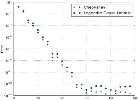
Ea  to implement the inextensible assumption in the literature. The domain is discretized by 31 Chebyshev nodes (N=30). The deflected shape of central axis is plotted as shown in Fig. 1. Fig. 2 shows the plots of the load versus the normalized horizontal and vertical displacements for the beam tip obtained by the spectral method compared to the solutions presented by Mattiasson[23]. Our results are in good agreement with Mattiasson’s solutions. The vertical displacements errors for N=2 to 50 are calculated (due to lacking the double precision analytical solution, we suppose that the solutions of N=50 are exact). The error convergence as a function of N is shown in Fig. 3 for both the Legendre Gauss-Lobatto approximation and the Chebyshev approximation. We note that for both polynomial base, the error decays exponentially until the rounding error is reached (when N=26, error<10-12).

[image:4.595.318.543.60.228.2]

The second benchmark problem involves the cantilever beam subjected to an end moment as shown in Fig. 4. The straight beam properties are L=2 and A=100. 31 Chebyshev nodes are employed, and the deformation exhibits a circle when M 100 and a half circle when M 50 . The Fig. 3. Convergence of the maximum errors for Chebyshev and Legendre Gauss-Lobatto collocation approximations to the cantilever beam under tip vertical force P=250.

Fig. 1. Deformed shape of central axis for straight cantilever beam under tip vertical force P.

Fig. 2. Load vs. tip displacement diagram for cantilever beam under tip vertical force P. u/L and w/L present the dimensionless horizontal and vertical deflection here and in Figures below. Data shown by circles and stars are taken from Ref. [19] while solid lines show our results.

IAENG International Journal of Applied Mathematics, 48:4, IJAM_48_4_08

[image:4.595.314.544.277.449.2] [image:4.595.311.548.515.687.2]

descent curve for 2-norm of errors with the increase of the number of nodes is shown in Fig. 5, and is compared to the exact solutions (perfect circle) for the tip moment of 100. We noticed that N=20 is exact enough to reach the rounding error in this case. Another observation is that for this particular problem, the Chebyshev approximation is more accurate than the Legendre Gauss-Lobatto approximation.

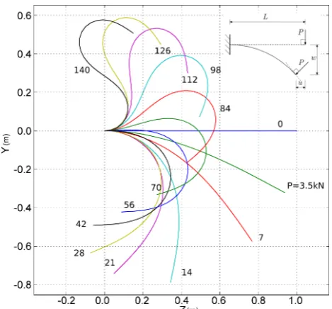
The third and fourth benchmark problems involve beams subjected to the follower load. This kind of problems has been studied by Argyris[24] and Nallathambi[11] using the finite element method and the fourth-order Runge-Kutta with shooting method separately. We use the same beam properties as in [11]. Figs. 6 and 7 show the resulting deformation profiles under different concentration forces. 31 Chebyshev nodes are used in the calculations and our results are in good agreement with the data reported in [24] and [11], as shown in Figs. 8 and 9. Furthermore, our results are in better agreement with the results of the fourth-order Runge-Kutta which is also a higher accuracy method compared to the finite element

[image:5.595.312.547.47.265.2] [image:5.595.49.291.142.319.2]

method; however, our method is more general and adaptable. More examples are presented below in different load and boundary conditions. In all examples, the discretization is carried out using 31 Chebyshev nodes. Fig. 10 shows the deflected shapes of the cantilever beam under the distributed Fig. 8. Load vs. tip displacement diagram for cantilever beam under follower force(showed in Fig.6). The solid lines and dashed line are from [11] and [20]. Fig. 4. Deformed shape of central axis for straight cantilever beam under tip

moment M.

[image:5.595.311.550.301.482.2]

Fig. 6. Deformed shape of central axis for straight cantilever beam under follower load P which is always orthogonal to the beam tip.

Fig. 7. Deformed shape of beam central axis for intrinsically curved cantilever beam under the tip force P which is always along the tangent of the curve tip.

Fig. 5. Convergence of the norm errors for Chebyshev and Legendre Gauss-Lobatto collocation approximations to the cantilever beam under tip moment M=100π.

IAENG International Journal of Applied Mathematics, 48:4, IJAM_48_4_08

[image:5.595.55.290.364.538.2]

vertical load q. One example of such situations is the large deformation of a very soft cantilever beam under gravity. The straight beam properties are the same as those of the first benchmark problem. We compare them to the results of the finite element code Calculix shown in Fig. 11. In the Calculix calculation, 20 three-node beam elements (element B32, all together 41 nodes) are used. The maximum relative deviation between the two solutions is less than 3%.

Fig. 12 illustrates an intrinsically curved beam deformed

[image:6.595.306.552.134.278.2]

with a fixed end and the other moving hinged end. This beam has the same properties as the beam in Fig. 7. When the hinged end moves horizontally with a certain displacement u, horizontal force P and vertical reaction N are provided to maintain the beam balance. Two reaction forces are shown in Fig. 13 as functions of the horizontal displacement.

A 3D large deformation example is obtained by applying the follower bending moment and torsion simultaneously on the free end of a cantilever beam with circular cross-section. According to Love[25], the curvature of the central-line is Fig. 10. Deformed shape of central axis for straight cantilever beam under

[image:6.595.59.285.161.326.2]

distributed vertical force q.

Fig. 9. Load vs. tip displacement diagram for intrinsically curved cantilever beam under follower force(showed in Fig.7). The solid lines and dashed line are from [11] and [20].

Fig. 14. Deformed shape of central axis for straight elastic beam with circle corss-section under tip bending moment and torsion.

[image:6.595.326.526.324.477.2]

Fig. 13. Horizontal force P and vertical reaction force N vs. horizontal displacement u of the hinged end.

Fig. 12. Deformed shape of central axis for intrinsically curved beam with a fixed end and the other moving hinged end.

Fig. 11. Load vs. tip displacement diagram for cantilever beam under distributed vertical force q (showed in Fig. 10). Circles and stars show the results obtained by Calculix while solid lines show the results obtained using our method.

IAENG International Journal of Applied Mathematics, 48:4, IJAM_48_4_08

[image:6.595.66.280.371.531.2] [image:6.595.310.548.521.707.2] [image:6.595.66.276.567.722.2]

constant and the beam will bend into the helical form. In the test, the elastic beam has the length of L=2, the bending stiffness of A=B=100, and the twisting stiffness of C=76.923. It can be seen from Fig. 14 that with the increase of both torsion and bending moments from 0 to 400, the number of helix turns increases.

V. OPEN COILED HELICAL SPRING

An important application of the flexible beam (or rod) in engineering is the open coiled helical spring with circular cross-section. The angle α between the coils and the plane perpendicular to the helix axis is not small, as shown in Fig. 15. The deformation of the wire produced by the axial compression load P includes twist and bending. The classical linear theory for the calculation of the spring deflection λ by the axial load is given in [26] as,

3 2 2

cos sin =

4 cos P

PD n

GI EI

  



 

 



 

 

(31)

where D is the diameter of the cylindrical surface containing the centerline of the spring, n denotes the number of coils and

β is the correction factor approximated as 1 for a very thin

wire. Some researchers further developed the nonlinear formula by introducing the correction of α [27]. Here, we calculate the deflection of one coil spring (n=1) by using the spectral method proposed in this paper.

The initial and intrinsic state of the spring is described by three Euler angles namely, the precession angle ψ=2scosα/D, the nutation angle θ=π/2-α and the spin angle φ=0 (the underlines denote the initial state). Four initial state Euler parameters are derived from the Euler angles as[28],

1

+

= cos cos

2 2

  

 , 2=cos sin

2 2

  

  ,

3=sin sin

2 2

  _

  , 4=sin cos

2 2

  _

  .

(32)

In the calculation, a modified first-type boundary condition is employed. We assume that one end of the wire is fixed at (0,0,0). The ending force F is generated by the compression load P, which is divided into many load steps and is applied according to (23). The ending moment for the ith load step is calculated as ( )



( 1) ( 1)

 



/ 2

i i i

x

D   L

  

M e r F , in which





3

sin 2 / =

D   and r

 

L is the position vector of the free ending. We also note that the nutation angles of both ends must be the same and ψ=0 at the fixed point, which induced,

( 1)

( ) 2 2

10 1 4

i i

L

  



  , _{3 0}0, ( 1)

( ) 2 2

20 2 3

i i

L

  



  , _{4 0}0.

(33)

The scheme proposed above is robust in the numerical tests and is easy to implement.

The parameters in the numerical test are listed as G=80 GPa, E=200 GPa, D=100 mm, α=10° and the diameter of the wire cross-section d is 5 mm. The helix height of one coil h is approximately 55.39 mm. The maximum compression load is applied as 100 N. According to the linear theory (31), the maximum deflection can reach 16.141 mm which is approximately 30% of the helix height.

Fig.16 shows the 3D plot of numerical results for one coil spring deflection. From the top to bottom, the applied loads are 0, 20, 40, 60, 80 and 100 N. In Fig. 17, a deflection comparison is performed for the classical linear theory, our numerical method and He’s equation. Fig. 17(a) shows that when the load is relatively small (1-10 N), all results agree with the linear theory very well. However, when the load become relatively large (10-100 N), as shown in Fig. 17(b), our numerical results (“circles”) depart from the linear straight line (“stars”) slightly by the nonlinearity from the variation of both α and D. The magnified views (c) and (d) Fig.15. Sketch of open coiled helical spring.

Fig.16. 3D plot of the one coil spring deflection.

(a) (b)

(c) (d)

Fig.17. Deflection comparison among different methods. Symbol “star” denotes the result from linear theory(31), “circle” denotes our numerical result and “triangle” is from the He’s equation. (c) and (d) are the zoom views of the square area in (a) and (b) separately.

IAENG International Journal of Applied Mathematics, 48:4, IJAM_48_4_08

show this result more clearly. We note that the results (“triangles”) from He’s equation (7) in [27] also depart from the linear straight line slightly but with the opposite direction compared to our result. The reason is that only the variation of

α is considered in his theory but the increase of the spring

diameter D. For example, Fig. 18 shows that the change of α and D with the increase of the axial load in our numerical test. When the load reaches 100 N, α and D become 0.12243 rad (7.015°) and 101.05 mm. If we substitute these values into the linear equation (31) to estimate the bound, the deflection is 16.576mm, near our numerical result of 16.435mm. However, when only α=0.12243 is substituted into the linear equation, the deflection is 16.065 mm, smaller than the classical linear theory result 16.141 mm, and the spring behaves stiffer. This is in agreement with the results as we have seen from Fig. 17(d).

VI. CONCLUSION

In this paper, we present an algorithm based on the polynomial collocation spectral method for the study of a thin elastic beam. Ten governing equations are discretized on the Chebyshev and Legendre Gauss-Lobatto points. Several benchmark problems and applications are tested to check the results and accuracy under different kind of loading conditions, intrinsic configurations and boundary conditions. The solutions are in good agreement with the results reported in the literature. The analysis also shows that the spectral method gives out extremely good quality with high precision on finite nodes. As the number of the nodes increases, the error decreases dramatically. This approach is more convenient to implement than traditional numerical methods, as the algorithm includes traditional routines that could simplify the coding task. With the advantages above, the method can be effectively applied in practice, especially in the fields that requiring rapid analysis with high accuracy.

REFERENCES

[1] T. P. Westcott, I. Tobias, and W. K. Olson, “Modeling self-contact forces in the elastic theory of DNA supercoiling,” J. Chem. Phys., vol. 107, no. 10, pp. 3967–3980, Sep. 1997.

[2] A. Goriely, M. Robertson-Tessi, M. Tabor, and R. Vandiver, “Elastic growth models,” Appl. Optim., vol. 102, pp. 1–44, 2008.

[3] H. Kang and J. T. Wen, “Robotic knot tying in minimally invasive surgeries,” in IEEE/RSJ International Conference on Intelligent Robots and Systems, Swiss Federal Institute of Technology Lausanne, Switzerland, 2002, vol. 2, pp. 1421–1426.

[4] M. Bergou, M. Wardetzky, S. Robinson, B. Audoly, and E. Grinspun, “Discrete elastic rods,” in ACM SIGGRAPH 2008, New York, NY, USA, 2008, p. 63:1–63:12.

[5] A. Theetten, L. Grisoni, C. Andriot, and B. Barsky, “Geometrically exact dynamic splines,” Comput.-Aided Des., vol. 40, no. 1, pp. 35–48, 2008.

[6] P. F. Pai and A. N. Palazotto, “Large-deformation analysis of flexible beams,” Int. J. Solids Struct., vol. 33, no. 9, pp. 1335–1353, Apr. 1996.

[7] G. H. M. Van der Heijden, A. R. Champneys, and J. M. T. Thompson, “Spatially complex localisation in twisted elastic rods constrained to a cylinder,” Int. J. Solids Struct., vol. 39, no. 7, pp. 1863–1883, 2002. [8] D. Q. Cao, D. Liu, and C. H. Wang, “Nonlinear dynamic modelling

for MEMS components via the Cosserat rod element approach,” J. Micromechanics Microengineering, vol. 15, no. 6, pp. 1334–1350, 2005.

[9] B. S. Shvartsman, “Direct method for analysis of flexible cantilever beam subjected to two follower forces,” Int. J. Non-Linear Mech., vol. 44, no. 2, pp. 249–252, Mar. 2009.

[10] M. Mutyalarao, D. Bharathi, and B. N. Rao, “Large deflections of a cantilever beam under an inclined end load,” Appl. Math. Comput., vol. 217, no. 7, pp. 3607–3613, 2010.

[11] A. K. Nallathambi, C. Lakshmana Rao, and S. M. Srinivasan, “Large deflection of constant curvature cantilever beam under follower load,” Int. J. Mech. Sci., vol. 52, no. 3, pp. 440–445, 2010.

[12] M. A. Langthjem and Y. Sugiyama, “Dynamic stability of columns subjected to follower loads: a survey,” J. Sound Vib., vol. 238, no. 5, pp. 809–851, Dec. 2000.

[13] K. M. Hsiao, W. Y. Lin, and F. Fujii, “Free vibration analysis of rotating Euler beam by finite element method,” Eng. Lett., vol. 20, no. 3, pp. 253–258, 2012.

[14] J. Song et al., “Fatigue crack propagation in BFRP reinforced RC beams based on fracture mechanics and golden ratio,” Eng. Lett., vol. 24, no. 4, pp. 449–454, 2016.

[15] B. D’Amico, H. Zhang, and A. Kermani, “A finite-difference formulation of elastic rod for the design of actively bent structures,” Eng. Struct., vol. 117, pp. 518–527, Jun. 2016.

[16] Y. Yang, I. Tobias, and W. K. Olson, “Finite element analysis of DNA supercoiling,” J. Chem. Phys., vol. 98, no. 2, pp. 1673–1686, 1993. [17] L. Greco and M. Cuomo, “An implicit G1 multi patch B-spline

interpolation for Kirchhoff–Love space rod,” Comput. Methods Appl. Mech. Eng., vol. 269, pp. 173–197, Feb. 2014.

[18] L. N. Trefethen, Spectral methods in MATLAB, vol. 10. Oxford: Society for Industrial Mathematics, 2000.

[19] Y. Liu and M. Wang, “A model and numerical study for coiling of Kelvin-type viscoelastic filament,” Mech. Res. Commun., vol. 70, pp. 17–23, Dec. 2015.

[20] Y. Liu, Z.-J. You, and S.-Z. Gao, “A continuous 1-D model for the coiling of a weakly viscoelastic jet,” Acta Mech., vol. 229, no. 4, pp. 1537–1550, Apr. 2018.

[21] D. A. Kopriva, Implementing Spectral Methods for Partial Differential Equations: Algorithms for Scientists and Engineers. Tallahassee: Springer, 2009.

[22] L. Mahadevan and J. B. Keller, “Coiling of flexible ropes,” Proc. R. Soc. Lond. Ser. Math. Phys. Eng. Sci., vol. 452, no. 1950, pp. 1679–1694, 1996.

[23] K. Mattiasson, “Numerical results from large deflection beam and frame problems analysed by means of elliptic integrals,” Int. J. Numer. Methods Eng., vol. 17, no. 1, pp. 145–153, 1981.

[24] J. H. Argyris and S. Symeonidis, “Nonlinear finite element analysis of elastic systems under nonconservative loading-natural formulation. part I. Quasistatic problems,” Comput. Methods Appl. Mech. Eng., vol. 26, no. 1, pp. 75–123, Apr. 1981.

[25] A. E. H. Love, A treatise on the mathematical theory of elasticity. New York: Dover Publications, 1944.

[26] S. P. Timoshenko, Strength of materials. Part II. Advanced theory and problems, 2nd edition. Lancaster: Lancaster Press, 1940. [27] Y. He, G. Zou, X. Pan, F. Zhang, and W. He, “Nonlinear theory and

experimental study of helical spring,” Eng. Mech., vol. 14, no. 2, pp. 56–61, Feb. 1997.

[28] H. Goldstein, Classical Mechanics, 2nd edition. Reading, Mass: Addison-Wesley, 1980.

Fig.18. Variation of α and spring diameter D with the increase of the axial load.

IAENG International Journal of Applied Mathematics, 48:4, IJAM_48_4_08