Abstract—Sensor deployment is one of the most important issues which affect the overall performance of a wireless sensor network (WSN). It is a challenging task to optimally deploy a limited number of sensors on three dimensional (3D) environments to maximize quality of coverage (QoC) and quality of network connectivity (QoN). In addition, when the environmental conditions are harsh and lossy, a robust sensor deployment strategy is needed. However, most of the studies on the subject are conveyed either by assuming two dimensional (2D) flat surfaces or put aside the overall WSN connectivity issues. In this study we have focused on deploying sensors on 3D terrains. The locations of sensors are determined with a multi-objective genetic algorithm (GA) by utilizing the novel wavelet transform (WT) based mutation operator. Also by determining the minimum spanning tree (MST) of the network, the minimum path-loss values and maximum coverage gain of the network are determined. The results of the simulation studies carried out on different types of terrains reveal that it is a robust and efficient method for sensor deployment on 3D fields.
Index Terms— sensor deployment, 3D environments, coverage, connectivity, genetic algorithm.
I. INTRODUCTION
ireless Sensor Networks (WSN) have been extensively studied in the last decade both in academic, military and civilian fields. Sensors in a WSN are deployed on a region to sense events and transmit the collected data to a base node for further operations [1]. Depending on the application demands, the localization of the sensors in order to achieve a desired coverage and connectivity is a major problem especially when the number of sensors at hand is limited.
Sensor deployment strategy has a significant effect on the performance of WSNs. However, the performance of the most sensor deployment models proposed in the literature are evaluated on planar surfaces, assuming random scenarios [2]. These models take into account a 2D free-space communication and a simple distance-based sensing model, where there are no obstacles or blocking between nodes and the sensed phenomena. In reality, sensor deployment takes place on 3D terrains where signals are blocked mostly due to the loss of line of sight (LOS) which results in a degradation in the communication and sensing tasks. A robust sensor deployment method have to take into account the geographical characteristics of the area of interest (AoI) because sensing coverage and communication accuracy in a realistic terrain environment highly deviates
1,2 Turkish Air Force Academy, Yesilyurt, 34149, Istanbul/Turkey
(1 Contact author e-mail: [email protected])
from that in a 2D assumed environment [2]. The density of obstacles between the transmitter and receiver antennas depends on the physical environment because fading and shadowing affects are caused by the surrounding obstacles [3]. Therefore, we present a more realistic model which considers the 3D terrain effects on both sensing and communication tasks and analyze the effect of the terrain structure by simulation studies carried out on various 3D terrains and for a 2D surface.
When deploying sensors on non line-of-sight (NLOS) spots (when a sensor is blocked by an obstacle), obtaining the optimum deployment scheme necessitates to take into consideration various objectives and constraints. Nevertheless, most of the sensor deployment methods in the literature are conveyed on 2D flat surfaces with putting aside some of the most important aspects such as, assuming unrealistic free-space communication, relying just on the Euclidian distance between sensors, regarding that there is always line-of-sight (LOS) between nodes and targets etc. Therefore, a more realistic model which also considers the 3D terrain effects on both sensing and communication objectives needs to be built into WSN applications. Hence, in this study, we have focused on an optimal deployment method over 3D sites to maximize quality of coverage (QoC) and network connectivity. The assessment of coverage quality bases on the sensing model which is utilized to measure the aggregated coverage of deployed sensors. A sensing model in WSNs is a mathematical function for the characterization of the sensor coverage utilizing distance and other environmental conditions [7]. The most commonly used sensing model is the binary sensing model where all the pixels within the detection ability of a sensor are marked as “1” and “0” otherwise. Probabilistic sensing model allows a more realistic modeling of sensor coverage probability [5-8].
Another issue in sensor deployment is the connectivity of the network [4]. It can be stated that the network is connected if and only if any active node can communicate with any other active node [4]. Network connectivity is also necessary to ensure that data packets are successfully delivered to the desired destination nodes and the loss of connectivity may cause unreachable sensors. Moreover, the routing algorithms for WSN periodically evaluate the minimum spanning tree (MST) of the network and construct route tables in order to find the best way to deliver its packet to a destination node [1]. In our case, we evaluate the quality of the network connectivity (QoN) of a deployment scheme by determining the MST of each deployment similar to the model which is proposed in [15]. Each 3D deployment can also be regarded as a weighted graph, where the weights reflect the quality of connectivity of every neighboring node
Wireless Sensor Deployment Method on 3D
Environments to Maximize Quality of Coverage
and Quality of Network Connectivity
Numan Unaldi1* and Samil Temel2
edge in regard to path-loss between node pairs. In this paper, in order to deploy sensors on 3D terrains to maximize both QoC and QoN, we utilize a multi-objective vector evaluated GA (VEGA) method which is regarded as a powerful multi-objective method [21]. As in our previous study [7], the mutation operator bases on the wavelet transform (WT). Also overall QoN of a deployment scheme is evaluated with a MST algorithm which also affects the fitness of a deployment scheme where the quality of received signal is determined with the log-normal shadowing path-loss model. The results show that our method provides promisingly effective results on 3D environments.
The paper is organized as follows: In Sections II, related work on sensor deployment methods is reviewed. In Section III, the methodology, some preliminaries and background information is presented and in Section IV, performance evaluations and an overview of simulation results are presented, respectively. The paper is concluded in Section V.
II. RELATED WORK
The deployment strategy is one of the fundamental steps which affect the overall performance of a WSN. In this section we briefly describe some of the sensor deployment methods which are basically conveyed on 3D environments with utilizing GAs. As stated earlier, sensors are deployed according to some given constraints such as terrain shape, sensor type, networking capabilities etc.
There are some examples in the literature which deal with deployment of minimum number of sensors and maximize the coverage on 3D environments. For example in [9], Wang et al. proposed a polynomial algorithm to find a solution to deploy some limited minimum number of sensors on a 3D field. A grid based approach and a greedy heuristic are introduced to determine the best placement of sensors. In [2], Arslan et al. investigates the effects of various 3D terrains on the performance of a WSN. They state that 2D assumption is unrealistic for the case of determination of sensor coverage and network connectivity. Although it is a valuable study to direct researchers to determine and characterize various terrain types such as rough, smooth etc. they neglect to propose a robust sensor deployment method.
In [10] Seo et al. proposes a new hybrid GA method with a new two-dimensional geographical crossover and mutation operator. The authors apply more real-world input factors such as sensor capabilities, terrain features, target identification etc. However, they do not propose solutions for 3D environments. A study which proposes a hybrid-evolutionary algorithm by taking into account multiple objectives can be seen in [8].
In another study, Bhondekar et al. proposes a GA based sensor deployment method with design parameters such as network density, connectivity and energy consumption [14]. A weighted sum approach has been used to aggregate all the optimization constraints and a single fitness function is formed which includes all the objectives. Also in [15], Marco proposes a multi-objective GA for sensor placement in Wireless Mesh Networks (WMNs) where individuals or solutions are represented by network graphs. In his method, a different approach to the problem is chosen by letting the algorithm to evolve toward the “good” graphs by using GAs. The problem is regarded as a kind of graph drawing problem where a GA is tailored to draw a graph in the plane
which satisfies the connectivity, the coverage percentage and the bit-rate of wireless links.
The coverage cavity mitigation is also a fundamental problem in sensor deployment [7], [13]. For the case of mitigating the coverage holes, Ghaffari et al. [13] proposed a divide-and-conquer deployment algorithm based on the triangular form that is executed on the three static sensors. Also in [7], Unaldi et al. proposes a more robust method which is based on WT in order to mitigate the coverage holes after an initial deployment of a number of sensors.
III. METHODOLOGY
In this study, we present a multi-objective GA method for deploying N sensors to maximize QoC and QoN. Initially, the terrain is divided into N sub-terrains and one sensor is placed randomly within a sub-terrain. As an example, with 16 sensors (N=16) the length of each gene will be 16 where the index of the array corresponds to a sub-terrain and the values of the array represents the location of the sensors as shown in Fig.1. Instead of using Cartesian coordinates, we use integer pixel numbering to represent locations. For representing the individuals, we use integer genes (arrays) of sensor pixel coordinates as shown in Fig.1. One individual gene of a population represents one deployment scheme on the terrain.
Sensor number 1 2 ….. 15 16
Pixel coordinate P1 P2 ….. P15 P16
Fig.1. Representation of individuals
An example of a 3D site is illustrated in Fig.2. In the figure, x and y axis represent the grid coordinates and z axis represents the elevations of the corresponding pixels where the red pixels represent the most elevated zones. In our proposed method, we consider a terrain, T, of size
pixels such as the one presented in Fig.2. Each sub-region is assigned with only one sensor and the length of each sub-region, , is equal to N. As an example, if the number of sensors is taken as 16 and the terrain size as 64 64 pixels (M=64), then the length of each sub-region is 16 pixels long
( 16). If Ti denotes the sub-region number, then we
have 16 sub- regions numbered from 1 to 16 (i=1,2,…16).
Fig. 2. A 3D site
A. Quality of Coverage (QoC)
[image:2.595.335.538.357.387.2] [image:2.595.305.559.571.682.2]regarded as closer to real world scenarios [5,7,19-20]. In the probabilistic sensing model, the sensed phenomenon is defined as p, the sensor is denoted as s, a predefined sensing range as sr and an uncertainty sensing detection range is defined as ur where ur<sr. If the sensed phenomenon p lies within (sr-ur) and there is LOS between s and p, then it is certainly sensed. If p lies out of the range from (sr+ur) or if there is no LOS (NLOS) between s and p then it is certainly not sensed. If p lies within (sr-ur) and (sr+ur) and if there is LOS between s and p, then the detection probability can be expressed with an exponential function which is stated in (1). The overall sensing probability of pixel i , reflects its probabilistic sensing degree. Here, ∆(s,p) denotes the 3D Euclidian distance between p and s.
,
1, ∆ ,
. , ∆ ,
0, ∆ ,
∆ , /2 (1)
The detection probability of a sensor within a predefined distance with different values of the α and β parameters yield different detection probabilities, which can be viewed as the characteristics of various types of physical sensors [20]. Throughout this study, sr is taken as 14 pixels and ur is taken as 2 pixels. Hence, the pixel distances up to 12 pixels (sr-ur) is definitely sensed with a probability of 1. Distances between 14 (sr-ur) and 16 (sr+ur) pixels, the phenomenon is sensed with a probability represented in (1). The distance greater than 16 pixels cannot be sensed. Consequently, the sensing probabilities of all the pixels are determined and the average of the overall values presents the QoC of a deployment on the 3D terrain.
B. Quality of Network Connectivity (QoN)
After deploying N sensors on a terrain, the sensors form a WSN which represents a connected weighted graph as shown in Fig.3. The weights indicate the radio propagation quality between two adjacent nodes. This graph can be represented as G(V,E) where V is the set of all the sensor nodes (vertices) and E represent the connections to the neighboring sensor nodes (edges). In this study we have utilized the log-normal shadowing path-loss propagation model to estimate the weights among sensor nodes which are scattered on a 3D environment [17]. In the log-normal shadowing path-loss model, the path loss in dB at distance d is given as
10 (2)
where PLF represents the free space loss and d0 is a reference distance. The path loss inherits the characteristics of free-space loss, and n is the path loss exponent which can vary from 2 to 6, based on the propagation environment, where n=2 is used for free space and higher values of n indicates there are more obstructions. Xσ denotes a Gaussian
random variable with a zero mean and a standard deviation of σ, and it takes into account the random shadowing effect. In order to reflect and mimic a 3D site, the free-space loss and path loss exponent values which were presented in [18] are utilized. In addition, in this study the average path-loss among two sensors is utilized as a network connectivity
quality measure, which is calculated by averaging the overall path-loss determined by adding up the path-losses in between the sensor nodes in the MST of the network. When given a graph GN, the MST of the graph can be evaluated with some greedy algorithms such as Prim’s Algorithm or Kruskal’s Algorithm. Both of these algorithms produce a spanning tree with weight less than or equal to the weight of every other spanning tree. More generally, a MST represents a spanning tree that has no cycles but still connects to every sensor node. There might be several spanning trees possible but a MST is the one with the lowest total cost. In order to evaluate the QoN of each deployment scheme, we evaluate the total signal loss in the corresponding MST.
C. Proposed Algorithm
In the simplest form, GAs select and replace all or some portion of the parents with the new offspring per each generation. To produce offspring, two parents are selected from the original population. They are recombined (crossovered) with one another and the results are mutated to form two children. In order to avoid premature convergence, which indicates stucking into local optima, mutation operators are used. For selection of the next generation, individuals are selected in proportion to their fitness (e.g. roulette wheel approach). Hence, if an individual has a higher fitness value, it is more probable to be selected. With an elitist approach, the fittest individual or individuals from the previous population are directly inserted into the next population.
Multi-optimization problems involve more than one objective function. If the objectives compete, the problem cannot be solved simultaneously. As stated earlier, in this study, we employ two independent objectives, one for QoC and the other one for QoN. Actually when deploying sensors on 3D terrains we would expect to maximize sensor coverage and minimize the path loss of the WSN. The coverage is maximized when sensors are deployed as far as possible to each other but the path loss is minimized when sensors are deployed as close as possible to each other. Hence, sensor deployment on 3D environments can be considered to be a conflicting optimization problem. In classical multi-objective GA methods, a weighted sum approach is utilized where a weight is assigned to each objective function in order to achieve a single scalar objective value. In this approach, the disadvantage lies in just choice of the weights [16]. Because of this, we employ a more robust and sophisticated multi-objective method, namely the vector evaluated GA (VEGA) method which is regarded as a more effective method [21]. In VEGA, the basic three-operator GA with selection, crossover and mutation is altered by performing independent selection cycles according to each objective. The selection method is separated for each individual objective to fill up a portion of the mating pool. Then the entire population is thoroughly shuffled to apply crossover and mutation operators. Specifically, at each generation, the population is divided into two equally sized subgroups because there are two objectives, namely QoC and QoN. The fittest individuals for each objective functions are selected, regular crossover and mutation operations are then performed to obtain the next generation.
In order to achieve a fair comparison, all the evaluated methods are started with the same initial deployment scheme and initially 20 random deployment schemes are formed which represent the initial population for the first generation. At each iteration, the population is divided into two equal sized populations randomly. Each sub-population is assigned a fitness based on a different objective. An elitist approach is used and the fittest parents in each sub-population are kept to be injected into the next generation. A temporary population is formed with the two sub-populations where the individuals are selected with fitness proportionate (roulette wheel) method. Afterwards, the temporary population is crossovered with the single point crossover method. The crossover point is selected randomly. Mutation operation is then performed on the populated children. The resulting population is assigned to be the next generation and for the next generation, the fittest parents are injected back into the generation.
Algorithm 1 Vector evaluated multi-objective GA (VEGA) method for sensor deployment on 3D terrains
1 : Create initial deployment;
2 : Determine the best individuals best1 & best2 according to objective1 & objective2;
3 : Divide the population into two sub-populations; 4 : for each sub-populationdo
4.1: Determine the fitness of eachindividual according to corresponding objective;
4.2: end for;
5 : Roulette wheel selection for each sub-population; 6 : Combine and shuffle sub-populations into temp- population;
7 : Perform recombination on temp-population;
8 : Perform mutation on temp-population;
9 : Next generation= temp-population;
10 : Inject best1 and best2 individuals into the next generation;
11 : If stop criteria is not satisfied, Goto step 2;
12 : Show results for objective1 & objective2;
D. Fitness Function
For the proposed method, we have two conflicting objectives one for maximizing the total sensing coverage and the other one for minimizing the total path loss in the network. The fitness function of the first objective, F , is evaluated to maximize the QoC of a deployment. Actually the second fitness function, F , represents a minimization objective but for the ease of calculation, we translate it to the problem of maximizing the QoN as will be explained later. The evaluation of each fitness function is presented in (3):
,
1/ ∑ (3)
where N represents the number of sub-terrains (which also equals to the number of sensors), ls represents the pixel length of a sub-terrain, s represents the location where the jth sensor resides on and p represents all the pixels in the sub-terrain. F is evaluated by taking the average of probabilistic sensing degrees, O , of all the pixels on a terrain which is derived from (1). In other words, we calculate all the sensing degrees (which are between "1" and "0") of the pixels on the terrain and take the average. As
F represents a maximization function, the bigger F values represent a better deployment scheme.
Evaluation of F is more straightforward. As stated in Section-III.C, each sensor deployment forms a 3D sensor network on a terrain. We find the MST and sum up all the path loss values, Pl of each deployment. Actually, we expect the path loss values to be between -80 dB and -100 dB. In order to turn QoN to be maximization objective we divide the aggregated Pl to -1.
E. GA Operators
In this study we used the single point crossover method owing to its simplicity and lightweight calculation. In recombining two parents, a random crossover point Pc is selected which represents the crossover point and after recombination, 2 new children are born. For the mutation operator we have utilized the guided walk mutation operator based on wavelet transform (WT) approach [7].
IV. RESULTS AND DISCUSSION
We have conducted simulations on two types of terrains, a smooth terrain and a rough terrain. The size of the terrains is 64x64 pixels and the number of sensors to be deployed is 16. Initially all the pixels in the terrain are numbered between 1 to 4096 and the terrains are divided into 16 equal length sub-terrains where the length of each sub-terrain is 16x16.
In this study, we propose a VEGA based multi-objective GA method where the deployment strategy mainly bases on the mutation operator employed. We present two different mutation operators one of which is the random mutation and the other is the WT based approach. With both of the two operators, the mutation operator bases on the movements (re-location) of sensors. With random mutation this movement is realized randomly. on the other hand with WT based mutation operator, the movements of sensors are guided movements that enforces the sensors to change its location towards to least covered zones.
In both of the mutation approaches, the decision that a sensor will be mutated is given with comparing a constant, Pm. At each iteration, a random number is generated and it is compared with Pm. If the number is less than or equal to Pm then the sensor deserves to be mutated, else it stays on its current position. In other words, mutation means movement of a sensor to a new pixel position. Throughout simulations, a movement of at least 1 and at most 4 pixels is employed. Also we make 10 simulation runs and present the average of the QoC and QoN results after 400 iterations. At each iteration the number of fitness evaluations is 20, which yields a total of 8000 fitness evaluations at each run.
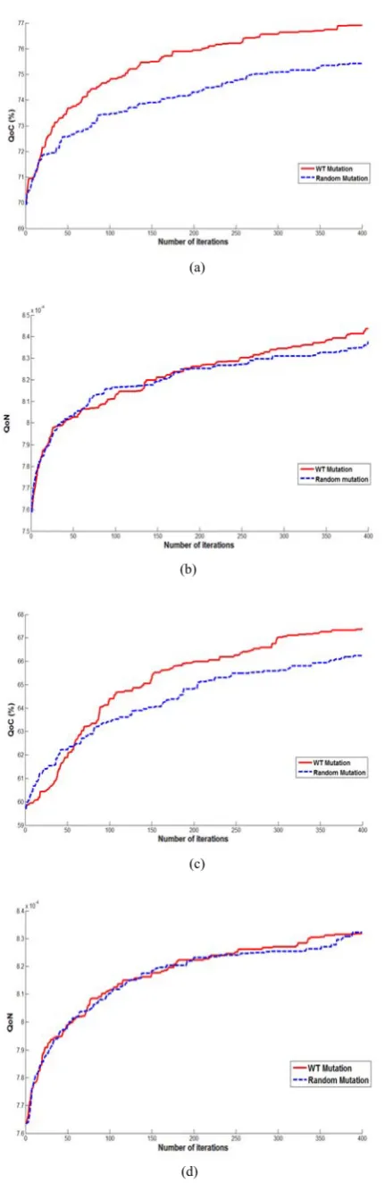
In Fig.3 (a), the maximum QoC values after 400 iterations (generations) with the random mutation method and WT based mutation method on a smooth terrain are shown. It can be seen from the figure that the maximum achievable QoC value with the random mutation method is 75 %. With the WT based method, a maximum QoC value of 77 % is achieved.
As shown in Fig.3 (b), after 400 iterations, the maximum QoN results for the random mutation method and the WT based method are 8.37x10⁻³ and 8.43x10⁻³ respectively.
(a)
(b)
(c)
(d)
Fig.3. Deploying 16 sensors with the random and WT based mutation
operators after 400 iterations a) The QoC results on a smooth terrain b) The QoN results on a smooth terrain c) The QoC results on a rough terrain b) The QoN results on a rough terrain
In Fig.3 (c), the maximum QoC values after 400 iterations on a hash terrain is shown. It can be seen from the figure that the maximum achievable QoC value with the random mutation method is 66.2 %. On the other hand, with the WT based method, a maximum QoC value of 67.5 % is achieved.
Also in Fig.3 (d), the maximum QoN results for the random mutation method and the WT based method are shown. After 400 iteration the maximum QoN reaches up to 8.33x10⁻³ for both methods. Since QoC indicates how well a
pixel on a terrain is covered, relatively slight improvement in its value is important as it denotes not only increased number of covered pixels but also increased quality of overall coverage. With the proposed algorithm, the QoN objective is also maximized which corresponds to minimizing the average path-loss in the MST of the network.
[image:5.595.63.279.48.711.2]
(a) (b)
Fig.4. QoC matrix on a smooth terrain a) after initial deployment b)
after 400 iterations.
In Fig.4, the QoC matrix of a smooth terrain is shown in gray scale after the first and last iterations. The black regions indicate non-covered pixels and white pixels indicate fully covered ones. It can be inferred from the figure that our method effectively determines the coverage holes in the matrix and effectively improves the QoC.
V. CONCLUSION
Deployment of limited number of sensors on 3D terrains in order to achieve maximum coverage and maximum network connectivity between sensor nodes is a challenging task. Although the literature for deploying on 2D environments is wide, studies on 3D environments are scarce. In the scope of this paper, we have developed a sensor deployment method which utilizes the novel WT based mutation operator in order to determine the coverage cavities and MST method in order to maximize network connectivity. For determining the network connectivity quality, we have evaluated the energy loss level with log-normal shadowing path-loss model. The approach followed in this paper bases on a multi-objective vector evaluated GA method and the performance results reveal that our algorithm will serve an effective and a robust method for sensor deployment on real world 3D sites.
REFERENCES
[1] Akyildiz, I.F.; Weilian Su; Sankarasubramaniam, Y.; Cayirci, E.; , "A survey on sensor networks," Communications Magazine, IEEE , vol.40, no.8, pp. 102- 114, Aug 2002
[image:5.595.315.546.259.375.2]Personal, Indoor and Mobile Radio Communications, 2008. PIMRC 2008. IEEE 19th International Symposium on , vol., no., pp.1-6, 15-18 Sept. 2008
[3] Tse, D.; Viswanath, P.; , “Fundamentals of Wireless Communication,” Cambridge University Press, 2005
[4] Türkoğulları, Y.B.; Aras, N.; Altınel, İ.K.; Ersoy, C.; , “Optimal placement, scheduling, and routing to maximize lifetime in sensor networks,” Journal of the Operational Research Society, vol.61, no.6, pp.1000-1012, June 2010
[5] Wu, C.H.; Lee, K.C.; Chung, Y.C.; , “A Delaunay Triangulation based method for wireless sensor network deployment,” Computer Communications, vol.30, no.14, pp. 2744-2752, Oct 2007
[6] Konstantinos P. Ferentinos, Theodore A. Tsiligiridis.; , “Adaptive design optimization of wireless sensor networks using genetic algorithms,” Computer Networks, vol.51, no.4, pp. 1031-1051, 14 March 2007,
[7] Unaldi, N.; Temel, S.; Asari, V.K.; ,“Method for Optimal Sensor Deployment on 3D Terrains Utilizing a Steady State Genetic Algorithm with a Guided Walk Mutation Operator Based on the Wavelet Transform,”Sensors, vol.12, pp. 5116-5133, 2012
[8] Topcuoglu, H.R.; Ermis, M.; Sifyan, M.; , "Positioning and Utilizing Sensors on a 3-D Terrain Part I—Theory and Modeling," Systems, Man, and Cybernetics, Part C: Applications and Reviews, IEEE Transactions on , vol.41, no.3, pp.376-382, May 2011
[9] Wang, J.; Zhong, N.; , “Efficient point coverage in wireless sensor networks,” Journal of Combinatorial Optimization, vol.11, no.3, pp.291-304, May 2006
[10] Seo, Jae-Hyun; Kim, Yong-Hyuk; Ryou, Hwang-Bin; Cha, Si-Ho; Jo, Minho.; , “Optimal Sensor Deployment for Wireless Surveillance Sensor Networks by a Hybrid Steady-State Genetic Algorithm” IEICE Transactions on Communications, vol.91, no.11, pp.3534-3543, 2008
[11] Joon-Woo Lee; Byoung-Suk Choi; Ju-Jang Lee; , "Energy-Efficient Coverage of Wireless Sensor Networks Using Ant Colony Optimization With Three Types of Pheromones," Industrial Informatics, IEEE Transactions on , vol.7, no.3, pp.419-427, Aug. 2011
[12] LoBello, L.; Toscano, E.; , "An Adaptive Approach to Topology Management in Large and Dense Real-Time Wireless Sensor Networks," Industrial Informatics, IEEE Transactions on, vol.5, no.3, pp.314-324, Aug. 2009
[13] Ghaffari, M.; Hariri, B.; Shirmohammadi, S.; , "On the necessity of using Delaunay Triangulation substrate in greedy routing based networks," Communications Letters, IEEE , vol.14, no.3, pp.266-268, March 2010
[14] A. P. Bhondekar, R. Vig, M. LalSingla, C. Ghanshyam, and P. Kapur.; , “Genetic Algorithm Based Node Placement Methodology for Wireless Sensor Networks,” Proceedings of the International MultiConference of Engineers and Computer Scientists, vol.1, 2009 [15] De Marco, G.; , "MOGAMESH: A multi-objective algorithm for node
placement in wireless mesh networks based on genetic algorithms," Wireless Communication Systems, 2009. ISWCS 2009. 6th International Symposium on , vol., no., pp.388-392, 7-10 Sept. 2009 [16] Konak A., Coit D. W., Smith A. E..; , “Multi-objective optimization
using genetic algorithms: A tutorial,” Reliability Engineering & System Safety In Special Issue - Genetic Algorithms and Reliability, vol.91, no.9,pp.992-1007, Sept. 2006,
[17] Rappaport T., “Wireless Communications: Principles and Practice,” Prentice Hall, 1996
[18] Gungor, V.C.; Bin Lu; Hancke, G.P.; , "Opportunities and Challenges of Wireless Sensor Networks in Smart Grid," Industrial Electronics,
IEEE Transactions on , vol.57, no.10, pp.3557-3564, Oct. 2010
[19] Chun-Hsien Wu; Kuo-Chuan Lee; Yeh-Ching Chung; , "A Delaunay triangulation based method for wireless sensor network deployment,"
Parallel and Distributed Systems, 2006. ICPADS 2006. 12th International Conference on , vol.1, no., pp.8, 2006
[20] Y. Zou and K. Chakrabarty, “Sensor deployment and target localization based on virtual forces,” Proc. IEEE INFOCOM, pp. 1293-1303, 2003.
[21] Patel, R.; Raghuwanshi, M. M., "Review on Real Coded Genetic Algorithms Used in Multiobjective Optimization," Emerging Trends in Engineering and Technology (ICETET), 2010 3rd International