Analysis of Algorithms Finding the Maximum Flow of a Planar Network

University of Canterbury Department of Computer Science

Honours Project Report

Analysis of Algorithms

Finding the Maximum Flow of a Planar Network Lynn Loader

Superv~sor A. M. Moffat October 1983

Abstract.

John H. Reif has recently developed an algorithm which finds the minimum cut of a planar network. This is a modification of an earlier algorithm presented by Itai and Shiloach and has a lower theoretical time bound than any other algorithm presented. This report compares the performance and discusses the implementation of Reif's and

Table of Contents

1 Introduction .. . . 1

2 Itai and Shiloach's Algorithm . . .

...

2.1 The Algorithm . . . . .. 6

2.2 To Show that the Algorithm Finds 2.3 Time analysis. • • • • • • 0 • • • • • • • • • • • • 3 Reif's Algorithm . . . 3.1 Discussion •.••• 3.2 The Algorithm .•. 4 Implementation ...•..••••...•••• 4.1 Generating Random Graphs •• 4.2 4.3 4.4 Design . . . . Data Structures. Program Design .•• the Minimum Cut ..

. . .

.

...

.

....

. .12 . . . . . . . 12

. . . . 14

. . . . 16

•. 16 . . . . 18

. . . 19

. .•••••••... 21

5 Results . . . 24

1 Introduction.

When a new algorithm to solve a problem is developed, an important part of the discussion of the algorithm is its efficiency with respect to time and space. The measure of the efficiency of an algorithm is often taken as the increase in the time taken for the algorithm to run as the size of the problem increases. This measure is a theoretical time measure and takes no account of the overhead incurred in actually implementing the algorithm ( foi example, two algorithms to solve the same problem may have O(n~) and O(n3 ) time bounds but the actual time taken to run may be 200n~ and 2~, although the O(n~ ) algorithm is theoretically better, in practice it is only better for problems where n > 100 ). Although the theoretical efficiency is important to consider, it is necessary to implement and test the algorithms to find the size problem for which the theoretically better algorithm is actually better, above this level the theoretically better algorithm will always be more efficient.

Many algorithms have been developed to find the maximum flow of a network such as Dinic's [Di] and Karzanov's [Ka] algorithms. Some of these algorithms have been developed to run on a special class of networks known as planar networks. Maximum flow problems turn up often in practice, for example to work out the time to pipe gas between two locations, given the topology of the network, the capacities of the pipe lines and the total amount of gas required.

This report looks at two algorithms for maximum flow in planar networks. Itai and Shiloach [IS] developed an algorithm which runs in

O(n~logn)

Shiloach's algorithm which runs in O(n(logn) ) ~ time, a saving of n/logn. The purpose of this report is to describe the implementation of Reif's algorithm and discuss the results obtained from testing, which show that Reif's algorithm is actually better than Itai and Shiloach's on the networks tested.

The rest of this section con~ains definitions and details of the notation used. Section 2 describes Itqi and Shiloach's algorithm, section 3 describes Reif's modifications to this algorithm. Section 4 is concerned with the implementation details of Reif's algorithm, section 5 gives the results of testing carried out on the two algorithms and section 6 contains comments on the results obtained.

Definitions.

1. A Graph G

= (

2. A Network is a graph in which a vertex s is called the source vertex and another vertex t is the sink vertex and a function C where C(e) is the capacity ( a non-negative real value ) of the edge e for each e in E.

3. A Flow in a network is a function F where F(e) is the flow through the edge e for each e in E.

The flow is subject to two conditions 1. 0 <= F(e) <= C(e) for each e in E.

2. For all v a member of v-{s,t} the sum of the flow out of v equals the sum of that into v.

The total flow of the network is the sum of the flow out of s which is the same as the sum of the flow into t.

4. The Maximum Flow is the flow F which is maximum while still obeying the flow rules.

5. Planar graphs ( or planar networks ) are graphs ( or networks which can be embedded into a plane. If a planar graph has n vertices then the maximum number of edges i t can have is 3n-6. This is derived from Euler's Theorem, which states that the number of vertices plus faces is equal to the number of edges plus 2. See [Ev] for this derivation.

Notation.

Throughout this report the following notation is used. All logarithms are assumed to be log base 2.

N stands for the number of vertices in a graph.

K stands for the number of vertices on the shortest s-t path used in both algorithms discussed.

V and v(i) also x(i) and f(i) in dual graphs ) are vertices. E represents an edge.

Ford and Fulkerson's Maximum Flow Minimum Cut Theorem.

Given a network N, an s-t cut is a set of edges that if removed from the network, divides it into two disjoint components, one containing s, the other t. The number of edges is assumed to be minimal, that is if any edge is removed from the cut, it would no longer be a cut. The value of a cut is the sum of the capacities of all the edges in the cut.

The maximum flow minimum cut theorem states that the maximum flow obtainable in any network is equal to the minimum value taken over all possible s-t cuts in the network. A proof of this theorem is given in

Note that while the value of the minimum cut will give the value of the maximum flow, it does not give the flow function F. Itai and Shiloach [IS] give two algorithms, one of which computes the minimum cut, the other gives the maximum flow function, given the value of this cut. This report concentrates on methods of finding the minimum cut and does not discuss how to obtain the flow function.

2 Itai and Shiloach's Algorithm.

Itai and Shiloach [IS] give an algorithm to find the minimum cut of an undirected planar network.

2.1 The Algorithm

Given an undirected planar network, the following algorithm will determine the minimum cut.

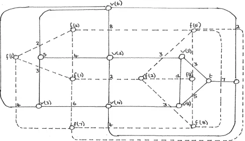
2.1.1 Find the Dual of the Network. The dual ( Gd of a graph G ) is a graph related to the original as follows

1. vertices in G are faces in Gd. 2. faces in G are vertices in Gd.

3. If an edge from vl to v2 bordering faces fl and f2 exists in G, there is an edge from fl to f2 bordering

faces vl and v2 in Gd.

4. If G is a network, the capacity of an edge in G becomes the cost of the intersecting edge in Gd.

/

/

-4l7.)_ ....

--"

---

--Fig 1. A Graph and its Dual.

"'

_{"' "'}

'

I

/

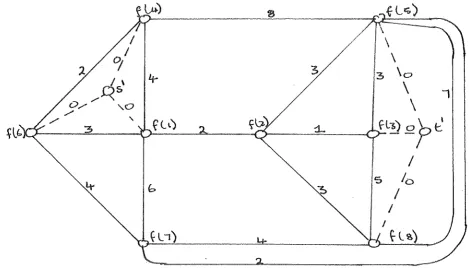
2.1.2 Once the dual of the network has been found it is augmented by

1. Adding two vertices, s' in face s and t' in face t.

2. Adding edges from s' to every vertex bordering face s and from t' to every vertex bordering face t. All these edges have a cost of 0.

:2

''"

3

\o

/~~

0 / '\.0 \

/

1

IL..)-/ _ _

...,:3~--'-f >---~----..~ "J---==---r:Jfl~)

2

~

~

Fig 2. The Augmented Dual.

2.1.3 The Shortest S-T Path.

I

s

/

I

I

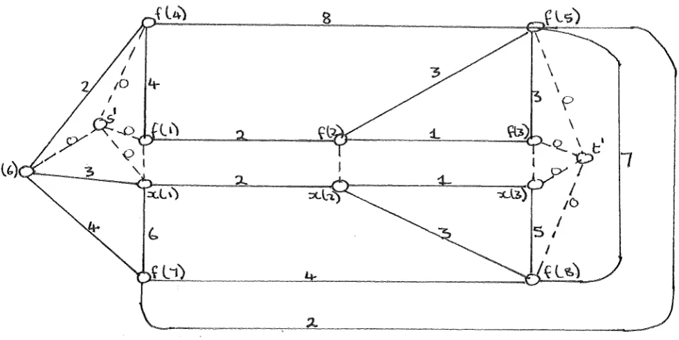
The shortest s-t path of this dual graph is found using Dijkstra's algorithm. The graph is then split along the path as follows :

1. For every vertex f(i) on this path, ( excepts' and t' a new vertex x(i) is added and if f(i)-f(j) is an edge on this path the edge x(i)-x(j) is added.

Fig 3. The Dual with the Duplicated S-T Path.

2.1.4 Find Cut Cycles in Gd. For each pair of vertices f(i) and x(i), the shortest path between them is found and the length of this path is recorded.

the graph. The

These paths are the minimum f(i) cut cycles in minimum of these cut cycles corresponds to the minimum cut in the original graph.

Fig 4. The Dual of Fig 3. with the Minimum f(i) Cut Cycles.

2.2 To Show that the Algorithm Finds the Minimum Cut.

The following two conditions, which hold for all planar undirected networks are necessary to show the minimum cut is found.

1. There is a 1-1 relationship between s-t cuts in G and the cut cycles in Gd. The cost of a cycle is the value of the cut.

2. The minimum cut cycle intersects the shortest s-t path and is therefore a minimum f(i) cut cycle for some f(i) on this path.

the cost of this cycle as the value of the minimum cut.

2.3 Time analysis.

For a graph with n vertices, the different steps of the algorithm have the following time complexities.

1. To construct dual O(m), where m

=

3. To find the shortest s-t ~ath O(nlogn) To add the extra vertices and edges O(n).

4. To find the shortest paths for each pair f(i),x(i) Worst case O(n~logn)

Usual case, if there are k vertices on the shortest s-t path, O(knlogn).

The total complexity of the algorithm is therefore O(n2logn) in the worst case and O(knlogn) in the general case, with step 4 being the dominant contributing factor to this time.

3 Reif's Algorithm.

Reif [Re] has developed an algorithm which follows the same structure as Itai and Shiloach. The first three steps are identical, and the modification to the fourth step is described below.

3.1 Discussion.

By modifying step 4 of Itai and Shiloach's Algorithm, Reif produced an algorithm with a general case running time of O(nlogklogn) and a worst case time of O(n(lognf ). His improvement was to notice that if

the shortest path between f(i) and x(i) was found, the shortest path between f(j) and x(j) for j <> i would not actually cross it as

1. It must cross in two place say at vertices vl and v2 2. The shortest path between vl and v2 is found by following

the shortest f(i),x(i) path from vl to v2.

Therefore any path including vertices vl and v2, but using another method to get from vl to v2 is not the shortest path and the shortest

f(j),x(j) path does not cross the shortest f(i),x(i) path, although they may have common edges.

vertices, to find the shortest paths for each of the middle vertices of these graphs takes O(aloga) and O(blogb) respectively.

The total time to find both these paths is O(nlogn) as aloga + blogb <= alog(a+b) + blog(a+b)

<= (a+b)log(a+b)

<= nlogn

This does not take into account the edges common to both graphs, Reif proves that these edges do.not increase the bound given above.

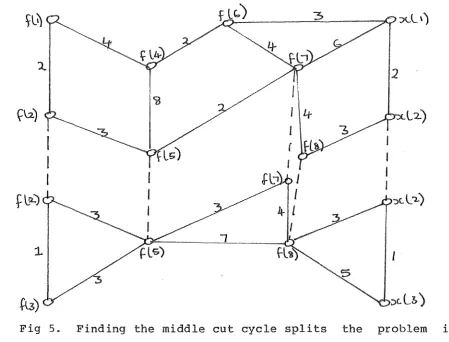
If this process is continued until each subproblem has only one shortest path to find, the depth of recursion is logk, with each level of recursion taking O(nlogn) time to compute making the total time to carry out the k searches O(nlognlogk).

Fig 5. Finding the middle cut cycle splits the problem into two smaller subproblems.

3.2 The Algorithm.

The algorithm is a recursive algorithm consisting of the steps

Procedure Calculate Shortest Paths ( upper, lower vertices ) • 1. middle := ( upper + lower ) mod 2.

3. Mark the shortest path from vertex 'middle' to vertex 'middle' + k as the current lower bound of the graph.

4. If middle <> upper then

Calculate Shortest Paths middle+l, upper ) .

5. Turn the lower bound found in step 3 to the current upper bound. 6. If middle <> lower then

Calculate Shortest Paths ( lower, middle-1 ) •

The algorithm is started by Calculate Shortest Paths ( 0, k-1 ) , where k is the number of vertices on the s-t shortest path, the vertices

o ..

vertices. The graph is expected in a slightly modified adjacency list format, as described below.

4 Implementation.

To test the actual running time of Reif's algorithm, the algorithm description in section 3.2 has been implemented. Itai and Shiloach's algorithm for this step has also been implemented as a check to see which is faster. The graphs used for the testing are generated with random edges, but each edge is given a cost of one. This enables the

shortest path algorithm to be replaced by a breadth first search and reduces the running time of each algorithm by a factor of O(logn)

making Reif's run in O(nlogk) and Itai and Shiloach's O(nk). This modification will not affect the comparative running time of the two algorithms. The algorithms are implemented in Pascal on a Prime 750.

4.1 Generating Random Graphs.

For effective testing to be carried out, a method of generating

random graphs had to be used. These graphs had to be subject to the conditions that they must be planar and that the shortest path between any two vertices represented as being on the s-t shortest path had to

4.1.1 Firstly the vertices are generated. The program requires the number of vertices (N) in the dual graph and the number of vertices on the shortest s-t path (k) as input. K vertices ( numbered 0 to k-1 ) are placed evenly along the line (0,0)-(0,1), another k vertices ( numbered k to 2k-l ) are placed evenly along the line

(1,0)-(1,1), these represent the vertices on the shortest s-t path and their duplicate vertices respectively. The other N-k vertices are given random coordinates in the unit square. The position of each vertex is tested as it is generated to make sure it is not 'close' to any other vertex, close being defined as having a euclidean distance less than 1/lOJN in this unit square.

4.1.2 Next the edges in the graph are generated by first constructing the s-t shortest path by linking the pairs of vertices v(i) to v(i+l), for all i in the range

o .•

the vertex. This list is sorted according to the euclidean distance between the vertices and the procedure tries to place edges to a random number within the bounds as input, of these vertices. Edges to the vertices closest to the vertex in question are tried first and inserted if they do not disrupt the planarity of the graph. Two edge records are created for each edge and one placed in the list of edges associated with each of the vertices the edge joins, each of which contains a pointer to the other. This is done to make the graph undirected.

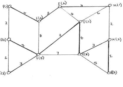
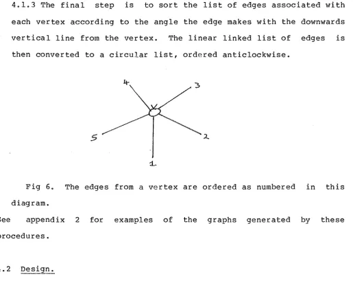
4.1.3 The final step is to sort the list of edges associated with each vertex according to the angle the edge makes with the downwards vertical line from the vertex. The linear linked list of edges is then converted to a circular list, ordered anticlockwise.

s

Fig 6. The edges from a vertex are ordered as numbered in this diagram.

See appendix 2 for examples of the graphs generated by these procedures.

4.2 Design.

This meant allowing direct access to those edges which form the minimum cut cycles, so the searching algorithm would only consider those edges in the current section of the graph. As a vertex can be on more than one cut cycle, more than one edge may need to be accessed. A list of edges on these cut cycles is stored for each vertex. A new record type is used to store the pointers to the edges concerned. A vertex may also be on both upper bounds and lower bounds at the same time, so two lists need to be kept, one list of upper bounds and one of lower bounds. New bounds are always put on the head of the lower bound lists, so the current lower bound is always the first on the list. The lower bounds must be converted to upper bounds in the reverse order to that in which they were generated, so the bound to be converted will also be the first on the list.

4.3 Data Structures.

The graph is stored as an array of vertices, each one of which points to a circular linked list of edges connected to the vertex. The edges are ordered anticlockwise and the vertex points to the first edge encountered from the downwards vertical line from the vertex. The maximum number of vertices is the constant max V which has been set to

3000.

The data structures used are :

Records. The names in brackets give the names of the record types in the Pascal declarations used.

Vertices ( node )

x, y

firste

father

real. Gives the cartesian coordinates of the vertex in the region O<=x<=l, O<=y<=l.

eptr. Points to the first edge in the list associated with the vertex.

eptr. Used by the searching procedure and is set to point to the edge between the vertex and

its father vertex in the edge list associated with the father vertex.

upper, lower : pathptr. Points to the list of records which indicate the edges from this vertex which form upper and lower ( respectively ) bounds.

Edges ( edgerec

source, dest integer. Indicate which pair of vertices the

pair

angle

nexte

edge joins. Source is always equal to the vertex associated with the record.

eptr. Points to the equivalent edge in the vertex 'dest' list.

real. Gives the angle in radians between the line (G[source] .x,G[source] .y) - (G[source] .x,O)

and the edge.

eptr. Points to the next edge in the edge list.

Paths ( pathrec ) edge

next_edge

eptr. points to the edge from the vertex on this path.

next V path_no

integer. Gives the next vertex on the path. integer. Gives the vertex number of the vertex the path starts from. This is not used by

the algorithm but allows the user to reconstruct the paths found.

The fields x,y in vertices, angle in edges and path_no in path are not used by the algorithm and, with the exception of path_no, are not set by it. They are included for user information and for the ease of getting the graph into the correct format.

The pointers used are EPTRs which point to an edgerec and PATHPTRs which point to a pathrec.

4.4 Program Design.

Parameters

G : an array of vertices, each pointing to their edge list this is the modified dual of the original graph.

N The number of vertices in the dual.

k The number of vertices on the shortest s-t path of the dual.

The total number of vertices expected is thus N+k. The vertices

O ••

The search is implemented as a breadth first search, following the usual algorithm with slight modifications to provide and use extra information needed and obtained by the algorithm.

The queue is a list of edge pointers, this enables the search to record which edge runs between the 'father' vertex and a son, so when a lower bound is set, the appropriate edge can be found directly instead of searching an edge list.

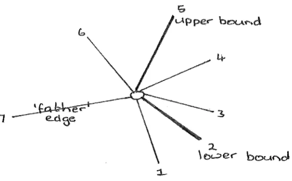
When edges are placed in the·queue, instead of placing all the edges associated with the vertex in the queue, a check is made to see if there are any upper or lower bounds associated with the vertex. If there is a lower bound, the first edge to go on the queue is the lower bound, otherwise the edge by which the veitex was reached. Edges are placed in the queue until the upper bound, if one exists, or the starting vertex is reached. Here the list is required to be circular, instead of linear. If the vertex ( v) is in the range k .. 2k-l only one edge is placed on the queue. If the search is started from vertex s then, if k <= v < s+k the edge v -> v+l is considered otherwise edge v -> v-1 is considered. This avoids the need to mark boundaries for edges in this range and also uses the fact that the shortest path from v to s+k is v,v+l,v+2 •• s+k (or v,v-l,v-2 •• s+k ).

1

Fig 7. Only the edges between the lower and upper bounds are looked at. Edges 1 and 6 do not need to be considered.

To mark the lower bound, the procedure starts at vertex 'middle+k' and traces back to vertex 'middle', at each vertex ( except middle+k ) a new pathrec is created and set to point to the same edge as the father field of the previous vertex. This procedure also records the length of the path.

To turn a lower bound into an upper bound, a procedure is called to trace along the lower bound starting from vertex 'middle', remove the first record from the list of lower bounds and place it at the head of the list of upper bounds.

5 Results.

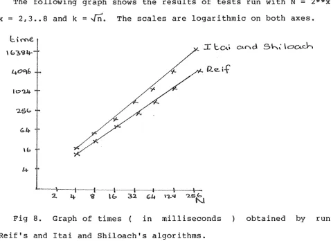
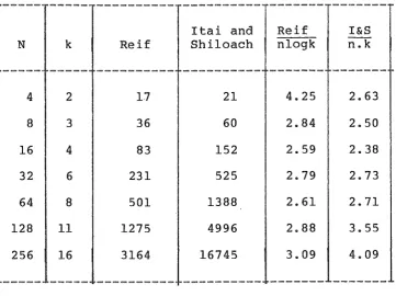
The following graph shows the results of tests run with N

=

=

=

Fig 8. Graph of times in milliseconds obtained by running Reif's and Itai and Shiloach's algorithms.

---

---

_---

_---

---

__

Itai and Reif I&S

N k Reif Shiloach nlogk n.k

---

---

--- ---

---4 2 17 21 4.25 2.63

8 3 36 60 2.84 2.50

16 4 83 152 2.59 2.38

32 6 231 525 2.79 2.73

64 8 501 1388 2.61 2.71

128 11 1275 4996 2.88 3.55

256 16 3164 16745 3.09 4.09

---

---

________

---

---

---Table 1. Times ( in milliseconds ) obtained from runs of Reif's and Itai and Shiloach's algorithms, varying N.

---

---

_{--- ---}

---Itai and Reif I&S

N k Reif Shiloach nlogk n.k

..

---

---

--- ---

---

---256 4 2156 4177 4.21 4.08

256 8 2806 8466 3.65 4.13

256 16 3164 16745 3.09 4.09

256 32 4106 35373 3.21 4.32

256 64 4979 72109 3.24 4.40

---

--- ---

___

---Table 2. Times obtained by running the algorithms, varying

The last two columns of the tables give an indication of how close the times obtained are to the theoretical time bounds. For most pairs of N and k these are reasonably constant, indicating that the times are close to those expected.

6 Cone

As can be seen from the consistently faster than

results obtained, Itai and Shiloach's.

Reif's algorithm ran The algorithm is more complicated than Itai and Shiloach and hence requires more programming effort, but once done achieves an elegant implementation. The data structure used is also more complicated. The overhead incurred by running this implementation and maintaining the data structure is surprisingly low, yielding good results on all the types of graphs tested.

This implementation shows that Reif's algorithm is a more efficient algorithm in practice as well as theoretically and so is a useful method of finding the minimum cut of a planar network. The implementation is more elegant than expected because of the method used to turn lower bounds into upper bounds. This turned out to be easier than originally anticipated.

Further Testing.

The following areas, which have not been implemented or tested, could be used for a more complete analysis of Reif's algorithm.

6.1 Generate graphs with edges having random capacity, and change the searching technique from a breadth first search to Dijkstra's shortest path algorithm, as would be needed in any practical implementation of the algorithm.

References.

[DI] Dinic E. A.

Algorithm for Solution of a Problem of Maximal Flow in a Network with Power Estimation.

Soviet Math. Dokl Vol 11 ( 1970 ) pp 1277-1280.

[Ev] Even S.

Graph Algorithms. Pitman, London, 1979.

[FF] Ford C. and Fulkerson D.

Maximal Flow through a Network.

Canadian Journal of Mathematics Vol 8 ( 1956 ) pp 399-404.

[IS] Itai Alon and Shiloach Yossi.

Maximum Flow in Planar Networks.

Siam Journal of Computing Vol 8 ( 1979 ) pp 135-150.

[Ka] Karzanov A. V.

Determining the Maximum Flow in a Network by the Method of Preflows.

Soviet Math. Dokl Vol 15 ( 1974 ) pp 434-437.

[Re] Reif John H.

Minimum S-T Cut of a Planar Undirected Network in O(nlog2 n) Time.

Siam Journal of Computing Vol 12 ( 1983 ) pp 71-81.

Appendix 1. Program Listings l.a Code for Reif's Algorithm.

subprogram reif;

Procedure search_graph }( var G : graph; v, N, k : vertex;

{

============

var

listptr

=

edge : eptr; next : listptr end ;

labelled : array [vertex] of boolean; head : listptr;

edge, place, stop : eptr; i : integer;

Procedure queue ( edge : eptr ) ;

{

---

---Places 'edge' into the queue of edges used by the search. } var temp, trace : listptr;

beg in

visited := visited + 1; new ( temp ) ;

temp~.next :=nil; temp~.edge := edge; trace := head;

if trace <> nil then begin

while trace~.next <> nil do trace := trace~.next;

trace~.next := temp end

else head := temp end ; { Queue }

Function fetch : eptr;

{

---

---Fetches ~he first edge from the queue and returns

a pointer to the edge. }

fetch := headA.edge; temp := head;

head := headA.next; dispose ( temp ) end ; { fetch }

Procedure Set limits

{

---

_---

This procedure sets the limits on the edges to be added to the queue maintained by the searching procedure. All the edges from START up to ( but not including ) STOP are to be added to the queue. If there is a lower bound from the vertex, START is set to this, otherwise START is set to the current edge. STOP is set to the edge following the upper bound, if i t exists, or

to the current edge. }

begin

with G[vl] do

if ( vl >= k ) and ( vl < 2*k then begin

if ( vl

=

stop := startA.nexte end

else begin

if up~er = nil then stop := edgeA.pair else

1

stop := upperA.edgeA.nexte;

if lower

=

start := lowerA.edge; end

end { set_limits } begin

for i := 0 to N+k-1 do labelled[i] := false; visited := 0;

new ( head ) ;

headA.next :=nil;

headA.edge := G[v] .firsteA.pair; while head <> nil do

begin

edge := fetch; with edgeA do

if not labelled[dest] then begin

labelled[dest] :=true; G[dest] .father := edge;

set limits (place, stop, dest ); repeat

queue (place);

place := placeA.nexte

until place

=

end end~

G [v] . father :

=

}

Procedure Minimum_cut ( var G

{

---

_---

This procedure finds the value of the minimum cut of a planar undirected graph using Reif's algorithm. It expects the dual of the graph for parameter G, with N vertices and k vertices on the shortest s-t path. It also assumes the graph has been split along this path. } var

i, length, min cut : integer;

path length : array [vertex] of integer; visited : array [vertex] of integer; time : array [vertex] of int~ger~ tl, t2 : integer;

Procedure lowertoupper ( v

{

============

Converts the path from vertex v to vertex v+k from being a lower bound to being the current upper bound by changing the pathrec records at the head of the 'lower' lists to being the

head of the 'upper' lists. }

var

i integer; temp : pathptr; beg in

i := v;

while i <> v + k do with G[i] do

begin

temp := lower;

lower := tempA.next edge; tempA.next edge :=upper; upper := temp;

i := upperA.next V

end;

-end; { lower to upper } Procedure marklower

{

---

_---

Puts the path from vertex v to v+k as the current lower bound on the graph by placing new pathrec records at the head of the

'lower' lists. It also calculates the length of the path, which

var i, j

temp begin

integer; pathptr;

i := v

+

if G[i] .father

=

=

while i <> v do begin

j := G[i] .father"'.source; new ( temp ) ;

with temp" do begin

next V := i; path-no := v;

edge-:= G[i] .father; next edge := G[j] .lower;

G[j]~lower := temp; , end;

i :

=

length := length + 1 end;

end ; { mark lower }

Procedure calculate ( lower, upper : integer ) ;

{

---

----~----Recursively calculates the shortest path from i to

i+k for all lower <= i <= upper, using a 'divide and conquer' technique. The values of all these shortest paths are stored

the array path_length. }

var

middle tl, t2 begin

mill ( t l ) ;

vertex; integer;

middle := ( upper + lower ) div 2; G[middle+k] .father := nil;

search graph ( G, middle, N, k, visited[middle] ) ; marklower (middle, path length[middle] ) ;

if middle < upper then calculate ( middle+l, upper ) ; lowertoupper ( middle ) ;

if lower <middle then calculate ( lower, middle-1 ) ; mill ( t2 ) ;

time[middle] := t 2 - tl; end; { calculate }

begin { minimum cut } mi 11 ( tl ) ;

for i := 0 to N+k-1 do begin

G[i] .upper

:=

calculate ( 0, k-1 ) ; mill ( t2 );

writeln ( 'Vertex Pathlength Edges searched Time' ) ; writeln (

'======

========== ============== ====' ) ;

writeln ( 0:4, path length[O] :10, visited[O] :12, time[O] :11); for i := 1 to k-1 do

begin

writeln ( i:4, path length[i] :10, visited[i] :12, time[i] :11); if path length[i] <-min cut then min cut:= path length[i]~

end; - -

-writeln ( 'The value of the minimum cut is ' , min cut : -4 ) ; writeln ( 'The total search time was ' , t2-tl:-8 );

l.b Code for Itai and Shiloach's Algorithm. subprogram breadth;

Procedure bfs ( var G

{

This procedure performs a breadth first search on

graph G, starting from vertex v. }

type

var

listptr = Alistmember; listmember = record

edge : eptr; next : listptr end ;

labelled : array [vertex] of-boolean; head : listptr;

edge, place, stop : eptr; i : integer;

Procedure queue

{

---

_---

Places the edge source to dest into the queue of

edges used by the search. }

var temp, trace : listptr; begin

new ( temp } ;

tempA.next :=nil; tempA.edge := edge; trace := head;

if trace <> nil then begin

while traceA.next <> nil do trace := traceA.next; traceA.next := temp

end

else head := temp end ; (* Queue *}

Function fetch : eptr;

{

---

---Fetches the first edge from the queue and returns

a pointer to the edge. }

var temp : listptr; begin

fetch := headA.edge; temp := head;

head := headA.next; dispose ( temp ) end ; ( * fetch *)

Procedure Set limits var start, stop : eptr; dest : vertex);

begin

start := G[dest] .firste; stop := start

end ; { set limits } beg in

for i := 0 toN do labelled[i] :=false; new ( head ) ;

headA.next :=nil;

head".edge := G[v] .firste".pair; while head <> nil do

begin

edge := fetch; with edgeA do

if not labelled[dest] then begin

labelled[dest] :=true; G[dest] .father := edge;

set limits (place, stop, dest ); repeat

end;

queue ( place ) ;

place := place".nexte until place

=

end

G[v] .father :=nil end ; (* bfs *)

Procedure Check search ( var G

{

---

_---

Runs Itai and Shiloach's minimum cut algorithm on graph G and outputs the k shortest paths and the time

taken to run the procedure. }

var i, j, count, tl, t2 : integer; begin

mill ( t l ) ;

for i := 0 to k-1 do begin

bfs ( G, i, N+k ) ; count := 0;

j := i + k; while j <> i do

begin

count := count + 1;

end~

writeln ( i : 5, count : 5 )~

end;

mill ( t2 ) ;

writeln ( 'Time to check search=', t2-tl 5 ); end; { check search }

l.c Data Structure Declarations.

const

max V

max E

=

3000; { max number of vertices }

=

9000; { max number of edges ( 3*max

type

vertex

=

O .. max V: { numbers for vertices }

eptr

=

Aedgerecs;

edgerecs

=

record { an edge }

source

integer;

dest

integer;

angle

real;

pair

eptq

nexte

eptr

end;

pathptr

pathrec

next V

"pathrec;

record { marks

: integer;

: integer;

eptr;

pathptr

an edge boundary }

path .... no

edge-next edge

end~-nodes

=

record { a vertex }

x, y

real;

father

eptr;

rste

eptr;

upper

pathptr;

lower

pathptr

Appendix 2. Examples of Random Graphs Generated for Testing

2.a N

=

~~r-._

I ,

I

I

!

2.c N = 128, k

=

}

·/