A sailwing vertical axis wind turbine for small scale applications

University of Warwick institutional repository: http://go.warwick.ac.uk/wrap

A Thesis Submitted for the Degree of PhD at the University of Warwick

http://go.warwick.ac.uk/wrap/4524

This thesis is made available online and is protected by original copyright. Please scroll down to view the document itself.

A SAILWING VERTICAL AXIS WIND TURBINE

FOR SMALL SCALE APPLICATIONS

Philip Scott Revell

A thesis submitted for the degree of Ph.D.

at the University of Warwick

CONTENTS

page no.

List of illustrations and tables _iv

Nomenclature xii

SUMMARY .XY

INTRODUCTION 1

1. PERFORMANCE THEORY FOR DARRIEUS TURBINES 10

1.1. Introduction 10

1.2. Analysis 13

1.2.1. The Effect of Reynolds Number 15

1.2.2. The Effect of Blade Aspect Ratio 16

1.3. Discussion 17

2. THE PERFORMANCE OF SAILWINGS IN DARRIEUS TURBINES 19

2.1. Introduction 19

2.2. Data 19

2.3. Results 22

2.3.1. Low Speed Performance 23

2.3.2. High Speed Perftrmance 24

2.3.3. The Influence of Aspect Ratio 24

244. Discussion 26

2.5. Conclusions 28

3. WIND TUNNEL TESTS OF SAILWINGS 30

3.1. Introduction 30

3.2. Experimental Apparatus 33

3.3. Test Details and Procedure 36

3.4. Results 39

-3.4.1. Solid Aerofoil and Rigid Trailing

Trailing Edge Tests 39

3.4.2. Elastic Trailing Edge Tests 41

page no.

3.5.

Conclusions 44

4. THE PERFORMANCE OF SAILWINGS IN DARRIEUS TURBINES

--A RE-ASSESSMENT 45

4.1. Introduction 45

4.2. Results and Discussion 45

4.3. Conclusions 50

5, A PROTOTYPE TURBINE 51

5.1. Introduction 51

5.2. Discussion 51

5.3. Design Details ₅₃

5.4. Prototype Theoretical Performance 57

5.5. Conclusions

₅₉

6. PERFORMANCE TESTS ON THE PROTOTYPE TURBINE 60

6.1. Introduction 60

6.2. Test Equipment and Measurements 61

6.2.1. Measurement of the Turbine Inertia 61

6.2.2. Measurement of Turbine Speed 62

6.2.3. Measurement of Windspeed 62

6.2.4. Measurement of the Trailing Edge

Tension 63

6.2.5. Test Method 64

6.3. Data Processing and Analysis 64

6.4. Results and Discussion 66

6.5. Comparison with other Turbines 68

6.5.1. Flow Curvature and the Prototype

Turbine 70

6.6. .Conclusions 72

7. THE PROTOTYPE TURBINE AS A WINDPUMP ₇₃

7.1. Introduction ₇₃

7.2. Turbulence in the Wind and Windpump Output 74

94

98

iii

page no.

7.4.

Performance Tests on a Diaphragm Pump

79

7.4.1.

Apparatus and Procedure 80

7.4.2.

Results and Discussion 81

7.5.

Testing of the Prototype Turbine under Load 83

7.5.1.

Arrangement and Predicted Performance

₈₃

7.5.2.

Tests, Results and Discussion

85

7.6.

Conclusions

88

DISCUSSION AND CONCLUSIONS

₈₉

REFERENCES

APPENDICES -- numbered according to chapter

Appendix 1 Derivation of some Equations & 6421z

artal,bsis

Appendix 2 Some Sample Computer Programs

₉₉

1. A single streamtube program

2. A single streamtube program

including allowance for varying Reynolds

Number and finite aspedt ratio

Appendix

3

₁₀₀

1. Relationship between the tension

coefficients Corand

CC,

2. Calibration of the leading edge

strain gauges

3. An additional test with a jib-sail

Appendix

5

₁₀₃

1. Modified expressions for an

inclined blade

2. The power absorbed by a...rotating

strut

page no.

Appendix

7

109

1. Turbulence in the wind

2. A simple theory for inertia flow

3. Pipe losses in the pump performance

tests

******************************

LIST OF ILLUSTRATIONS AND TABLES following

page no.

Fig.0.1. Various types of windmill

₉

Fig.1.1. Section through a Darrieus turbine showing a

blade element at various positions 12

Fig.1.2. Actuator disc model of the turbine 12

Fig.1.3. Variation of the angle of incidence with

azimuthal angle at low tip speed ratios 12

Fig.1.4. Rate of change of angle of incidence vs.

azimuthal angle 12

Fig.1.5. Variation of angle of incidence along blade

chord 12

Table 2.1. Details of sailwings 20

Fig.2.1. Lift and drag coefficients used for the solid

aerofoil (NACA0012), taken from Shankar

(1976)

21

Fig.2.2. Lift and drag coefficients for Sailwing 1

(from Robert and Newman,

1979)

21

Fig.2.3. Lift and drag coefficients for Sailwing 2

(from Robert and Newman,

1979)

21

Fig.2.4. Lift and drag coefficients for Sailwing 3

(from Robert,and Newman,

1979)

21

Fig.2.5. Angle of incidence vs. azimuthal angle at low

following

page no.

Fig.2.6. Ratio evs. azimuthal angle at low tip speed

ratios

22

Fig.2.7. Tangential force and torque coeffs. vs.

azimuthal angle, solid aerofoil 25

Fig.2.8. Tangential force and torque coeffs. vs.

azimuthal angle, Sailwing

1

25

Fig.2.9. Tangential force and torque coeff. vs.

azimuthal angle, Sailwing 2 25

Fig.2.10. Mean torque coefficient vs. tip speed ratio 25

Fig.2.11. Mean torque coefficients vs. tip speed ratio

for sailwing 1 with varying scale 25

Fig.2.12. Power coefficient vs tip speed ratio,

solid aerofoil 25

Fig.2.13. Power coefficient vs. tip speed ratio,

Sailwing 1 25

Fig.2.144 Power coefficient vs. tip speed ratio,

Sailwing 2 25

Fig.2.15. Power coefficient vs.

tip speed ratio,

Sailwing

3

25

Fig.2.16. Mean torque coefficient vs. tip speed ratio,

solid aerofoil, varying aspect ratio 25

Fig.2.17. Power coefficient vs. tip speed ratio for

solid aerofoil with AZ=4 25

Fig.2.18. Power coefficient vs. tip speed ratio for

solid

aerofoil

with AZ =8 25

Fig.2.19. Mean torque coefficient vs. tip speed ratio,

Sailwing 1, varying aspect ratio 25

Fig.2.20. Power coefficient vs. tip speed ratio for

Sailwing 1 with

AZ. 8

25

Fig. 2.21. Power coefficient vs. tip speed ratio for

vi

following

page no.

Fig.2.22. Power coefficient vs. tip speed ratio for

Sailwing 3 with AZ = 4 25

Fig.2.23. Power coefficient vs. tip speed ratio for

Sailwing . :3 with A =

8

25

Fig.3.1. Experimental set-up 35

Table 3.1. Test details 35

Fig.3.2. View of experimental set-up with the tunnel

wall removed 35

Fig.3.3. Arrangement of the flexures and strain gauge

bridges 35

Fig.3.4. Rigid trailing edge 35

Fig.3.5. Blade geometry for elastic trailing edge tests 35

Fig.3.6. Comparison of lift and drag coefficient with

published data, NACA0012 • 35

Table 3.2. Fabric elasticity 36

Fig.3.7. Tangential force coefficient vs. angle of

incidence for NACA0012 aerofoil 43

Fig.3.8. Radial force coefficient vs. angle of incidence

for NACA0012 aerofoil 43

Fig.3.9. Tangential force coefficient vs. angle of

incidence for canvas sailwings 43

Fig.3.10. Tangential force coefficient vs. angle of

incidence for nylon sailwings 43

Fig.3.11. Tangential force coefficient vs. angle of

incidence for 'Dacron' sailwings 43

Fig.3.12. Radial force coefficient vs. angle of

incidence for canvas sailwings 43

Fig.3.13. Radial force coefficient vs. angle of

incidence for nylon sailwings 43

Fig.3.14. Radial force coefficient vs. angle of

vii

following

page no.

Fig.3.15. Lift coefficients for canvas sailwings 43

Fig.3.16. Lift coefficients for nylon sailwings 43

Fig.3.17. Lift coefficients for 'Dacron' sailwings 43

Fig.3.18. Drag coefficients for canvas sailwings 43

Fig.3.19. Drag coefficients for nylon sailwings 43

Fig.3.20. Drag coefficients for 'Dacron' sailwings 43

Fig.3.21. Lift and drag coefficients, canvas sailwings 43

Fig.3.22. Lift and drag coefficients, nylon sailwings 43

Fig.3.23. Lift and drag coefficients, 'Dacron' sailwings 43

Fig.3.24. Results from Buehring (1977) 43

Fig.3.25. Tangential force coefficient vs. angle of

incidence for sailwings with an elastic trailing

edge 43

Fig.3.26. Radial force coefficient vs. angle of

incidence for sailwings with an elastic trailing

edge 43

Fig.3.27. Lift coefficients -elastic trailing edge 43

Fig.3.28. Drag coefficients -elastic

trailing edge

43

Fig.3.29. Induced tension coefficient vs. angle of

incidence 43

Fig.3.30. Induced tension coefficient vs. angle of

incidence 43

Fig.4.1. Tangential force and torque coeffs. vs.

azimuthal angle -Calp 49

Fig.4.2. Torque coefficient vs. tip speed ratio

-solid aerofoil 49

Fig.4.3. Torque coefficient vs. tip speed ratio from

data for canvas sailwings 49

Fig.4.4. Torque coefficient vs. tip speed ratio from

viii

following

page no. Fig.4.5. T orque coefficient vs. tip speed ratio from

data for 'Dacron' sailwings 49

Fig.4.6. Variation of the ratio y . with azimuthal angle 49

Fig.4.7. Power coefficient vs. tip speed ratio,

single streamtube program, data from test Nylw 49

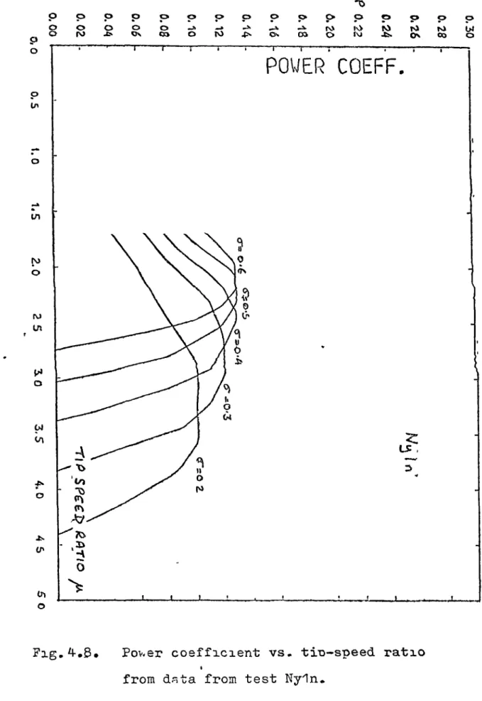
Fig.4.8. Power coefficient vs. tip speed ratio,

data from test Nyln 49

Fig.5.1. Some possible arrangements for a sailwing

turbine 56

Fig.5.2. View of the prototype turbine 56

Fig.5.3. Dimensions of a single sail 56

F ig.5.4. An inclined turbine blade 58

Fig.5.5. Torque coefficient vs. tip speed ratio

-prototype turbine, predicted 58

Fig.5.6. Predicted torque and power coefficient curves

for the prototype turbine 58

Fig.6.1. View of the wind turbine test site 71

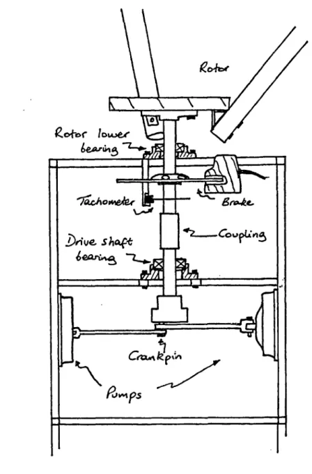
Fig.6.2. Diagram of the tachometer arrangement 71

Fig.6.3. Schematic plan of the prototype turbine test

arrangement 71

Fig.6.4. Rotor and windspeed vs. time during a typical

test run ₇₁

Fig.6.5. Torque and power coefficients vs. tip speed

ratio with a nylon trailing edge 71

Fig.6.6. Torque and power coefficients vs. tip speed

ratio with a wire trailing edge 71

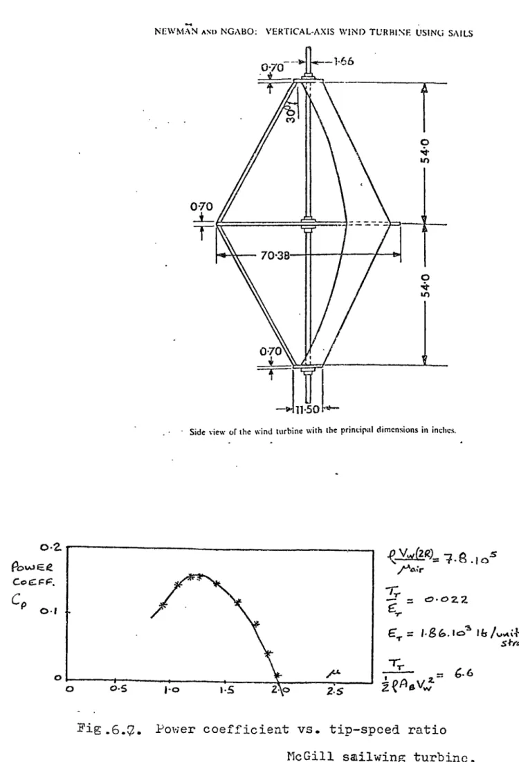
Fig.6.7. Power coefficient vs. tip speed ratio,

McGill sailwing turbine (Newman and Ngabo 1 1978) 71

Fig.6.8. Power coefficient vs. tip speed ratio,

ix

following

page no.

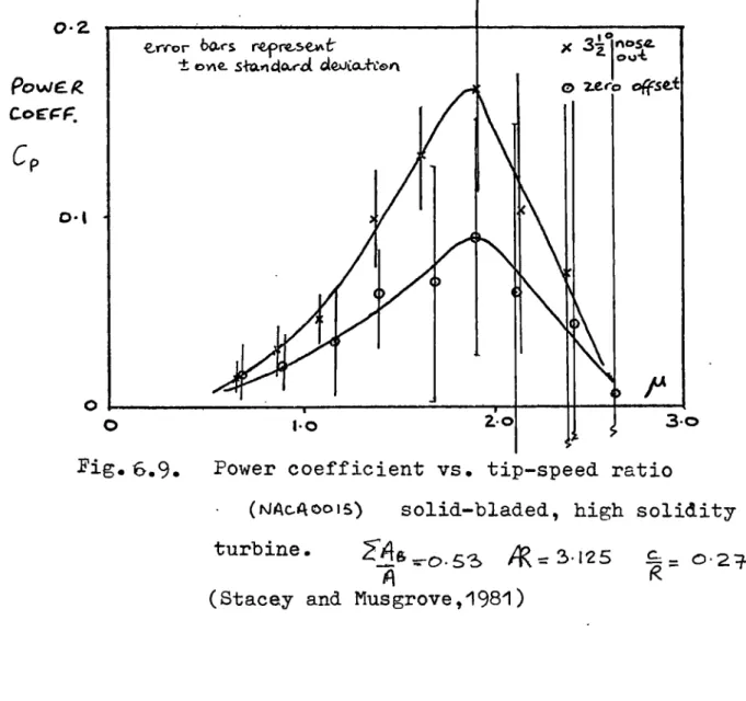
Fig.6.9. Power coefficient vs. tip speed ratio,

solid bladed, high solidity turbine

(Stacey and Musgrove11981) 71

Fig.6.10 An approximation to the virtual blade profile 71

Fig.6.11. The variation of virtual pitch angle and virtual

virtual camber ratio with azimuthal angle at low

tip speed ratios 71

Fig.7.1. A spectrum of the horizontal windspeed

(van der Hoven 1 1957)

₇₇

Fig.7.2. Some typical recordings of windspeed at the

test site

₇₇

Fig.7.3. Turbine and load torque curves

₇₇

Fig.7.4. Windspeed and rotor speed vs. time with various

load torques

₇₇

Fig.7.5. Wind power and power absorbed by various loads

vs. time

77

Fig.7.6. Theoretical curve for dimensionless flow vs.

dimensionless speed 80

Fig.7.7. _{Arrangement for pump performance tests} 80

Fig.7.8. Pump test rig and tensioner arrangement 80

Fig.7.9. Overall efficiency, average torque and

volumetric efficienCy vs. speed for diaphragm

pump 82

Fig.7.10. Overall efficiency, average torque and

volumetric efficiency vs. speed for diaphragm

pump 82

Fig.7.11. Water mass flow rate vs. pump speed. 82

Fig.7.12: Dimensionless flow vs. dimensionless speed

—comparison of measurements and theory 82

Fig.7.13. Assumed flow velocity curves for a diaphragm

following

page no.

Fig.7.14. Torque vs. speed curves for the turbine and a

pair of pumps 82

Fig.7.15. Arrangement of the pump drive shaft 87

Fig.7.16. Predictions for rotor speed and water flow

rate for the prototype windpump 87

Fig.7.17. A typical recording of ....turbulent wind 87

Fig.7.18. Section through air snifter 87

Fig.7.19. Rotor and windspeed vs. time -two pumps 87

Fig.7.20. Rotor and windspeed vs. time -one pump 87

Fig.A1.1. The relationship between the lift, drag and

tangential force coefficients 98

Fig.A1.2. The relationship between the lift ldrag and

thrust coefficients

98

Fig.A3.1. Loads in the sailwing frame due to

pre-tension in the sail 100

Fig.A3.2. Calibration load 101

Fig.A3.3. Mounting arrangement for jib sails 102

Fig.A3.4. Tangential force coefficient vs. angle of

incidence for a canvas sailwing with and without

a jib sail 102

Fig.A5.1. To define the nomenclature used in deriving

expressions for an inclined blade 104

Fig.A5.2. Estimated change in the power coefficient due t

to the power absorbed by the three struts of the

prototype turbine 105

Fig.A6.1. Calibration curve for the tachometer circuit 108

Fig.A6.2. Calibration curve for anemometers 108

Fig.A7.1. Auto-correlation function and power sDectral

xi _following

page no.

Fig.A7.2. Theoretical flow velocity curves for full

and partial inertia flow 111

Fig.A7.3. Inlet and outlet valves to the pump 116

Fig.A7.4. Assumed flow velocity curve for the diaphragm

pump 116

Fig.A7.5. Half-sine curve with mean value giving the

xii

NOMENCLATURE

G. Slope Ciloco prior to stall

M. Slope glee prior to stall

4 Turbine swept area

As Blade plan area ,

Ai, Cross-sectional area of inertia pipe

Af Piston area of reciprocating pump

Aspect ratio of aerofoil = 6,/c

ii Length of aerofoil blade

C Blade chord or strut chord

Ci, _{Drag coefficient = Drag force/Wie,VR2}

C; Thrust coefficient = Retarding force on airstream/10v

C. Lift coefficient = Lift force/AV:

C lot Induced drag coefficient = C,11/Trick

Cp Power coefficient _{= PiikANC3}

CI;Power coefficient = P/11Z A V3

cp.,. Membrane tensiori coefficient = Pr / -1? V,:-

c

C

Q Torque coefficient = Turhivle. -Forcpue P2-. A V,,,,2" g

Cs2 Radial force coefficient = C.i.c.osoc.4- Czszeloe

'LW

Cis Mean torque coefficient = lid CA,2 "

0

Ci. Tangential force coefficient .

Cist,,..c-C6c0s04-(C1_{4)Instantaneous torque coefficient for a blade = 1V-IRA8vIR.}

CI Trailing edge tension coefficient = T.r/J-z-16vgt

C. A Induced tension coefficient

= chordwise component of tension induced/1(c ot DictmetP-r _{oC teck.clie,g ectse...}

ciD Elemental drag force

olL Elemental lift farce

I i. Diameter of the inertia pipe

e. Ratio: force per unit width/strain, for membrane

Ratio: force/strain, for trailing edge line

C

Frequency

P

. Retarding force on windstream

8 Acceleration due to gravity

h, Head Loss

Head of water

3

Moment of inertia

k Constant =

04a.

k non-dimensional head loss coefficient h,43.

L Suspension length

L. Length of inertia pipe

m Turbine mass

Water mats flow rate

n Number of turbine blades

f Dynamic pressure or axis co-ordinate

P Power produced by turbine

P Membrane pre-tension per unit width

PwPower in the wind

Ratio:

Ve/V

Q Volumetric water flow rate

ri

Blockage ratio in wind tunnel cscv, 04

• s wieres

R Rotor radius

Re Pump crank length

Ru Auto-correlation function

Rs Suspension radius

ke

Reynolds number = V/12.c4tair

or

"LLD . /

,i1)

-r

Torque

T.T. Pre-tension in trailing edge

u, Water flow velocity, or a length

v- Fluctuating component of windspeed

V

iz Relative windspeed Vw Free windspeed

LA) A length

V/

Work done

x Maximum hollow in trailing edge curve

Ratio:

7./g0,11

/

Z

Vertical distance along turbine axis

doZ

Angle of incidence of relative wind to blade chord

oe Effective angle of incidence, with finite apsect ratio_4ff

A

Virtual pitch angle

e

Angle of inclination of turbine blade to the vertical,

or piston angular position

& Dimensionless speed

6

Blockage factor

7voL

Volumetric efficiency

El' Azimuthal angle (blade angular position)

X

Piston angular postion

/A Tip speed ratio

_{= RS1/Vw}

,1

2 Tip speed ratio

₌

Rn-lV

/A

ar Viscosity of air it-. 1-e2-10 KA30AAS

1) Virtual camber ratio or ieZne-ikka-t-c. vZscostk of watcr

1/4.S Dimansionless flow

=

Y/vo i. CS.

IL

Air density A.:, 1- 2_

_kg

/ 3nAn,

.

1 Mass of membrane per unit area

Water density e.: 103 k./w,3

cr Turbine solidity

-A/102A

le Time interval

05(4

Power spectral density •

S/ Angular velocity

SUMMARY

The use of sailwing aerofoils in vertical axis wind turbines has been investigated. It was anticipated that this could make vertical axis turbines more suitable for water pumping and that this might help to meet the need for a cheap pump for irrigation existing in many parts of the world.

A numerical analysis of the theoretical performance of such a turbine, using existing aerodynamic data for simply constructed sailwings, has been made. This gave an improved understanding of the operation of such turbines but showed a need for further aerodynamic data. Some new wind tunnel tests

of sailwings are described in which the effect of pre-tension was investigated and four different fabrics were tested.

The results are presented for angles of incidence up to 180 degrees and compared with previous data.

With the fresh data, new performance predictions were made which led to the design of a two metre diameter prototype turbine. This used an inclined blade configuration with a guyed top bearing. Canvas was used for the sails. It was predicted that the turbine performance would be significan-qy affected by windspeed.

The turbine was built and later tested in the open air. An acceleration test method was used and the tests generally confirmed the predictions. The averaged starting torque

coefficient was about 0.07; the averaged peak power coefficient was about 0.1 at a tip speed ratio of 1.4.

Consideration has been given to improving windpump system efficiency by improving the gust energy utilisation. Some

tests of a diaphragm pump are described in which inertia flow effects were used. A pair of such pumps were later connected to the prototype turbine. A number of problems were encountered and satisfactory operation was not achieved in the time

INTRODUCTION

This thesis is the result of some research into the

potential for using sailwing aerofoils in vertical axis

wind turbines. It was anticipated that such a turbine could

be suited to low lift water pumping, particularly for

irrigation, in Third World countries.

There would not seem to be any doubt about the

considerable potential of renewable energy technologies in

meeting the energy needs of development. The people of

the Third World, in fact, already meet the majority of their

energy needs from solar-energy and, when wood, food, crop

residues etc. are included, the energy use is much higher

than might be supposed. However, as shown by Makhijani (1976),

the efficiency of energy usage is generally very low and

it is probably by increasing the efficiency of energy use

that some of the most pressing energy needs of the poor

may best be met in a short time.

Basic in an increase in the energy use efficiency,

is an increase in the productivity of agriculture. Properly

managed, an increased energy input to agriculture, in the

form of fertiliser, irrigation and machinery, may increase

the net energy output per unit of land; i.e. crops may

capture more solar energy. Hence, subsistance agriculture

may be transformed into one producing surplus energy, in

the form of food and crop residues, to other parts of the

If irrigation is available then it may be possible

to harvest several crops a year where rainfall may be

largely confined to one season and crop failure due to

erratic rains may be avoided. For widespread irrigation

a source of energy other than that of human labour or

draught animals is necessary, particularly if the land is

to be productively cultivated in the dry season. The use

of windpumps seems an obvious solution in areas where a

suitable wind regime exists.

Makhijani suggests some criteria for windmill design

in the rural Third World:

"1. Low cost; the total cost should be less than POO

and preferably less than 100 so that small farmers and

others who may need a source of power for cottage industries

would be able to afford it,

(1976

prices)

2. It should have sufficient power to enable irrigation

of a small plot to i a hectare) and a power take off

to enable it to perform other functions such as sugar cane

crushing. The size of the windmill therefore depends on

the source and quantity of water needed,

3. It should be made of loc . al materials as far as

possible and with local skills (i.e. those available in

a small village). Among the reasons for establishing this

criterion are: i. low capital input and high labour intensity,

accessibili .py of the technology to the

poor,

iii. ease and quickness of maintenance and

repair when required,

satisfaction in ones work and control of it,

V.

high labour productivity,

4. It should be stable under adverse weather conditions,

5. It should have a high starting torque so that

auxilary starting devices are not needed."

The quantity of water required for irrigation depends

on the climate, the crop and its stage of growth and the

efficiency of the water distribution system. Average

requirements seem to lie between 40 and 100 m 3 /ha per day

(Stern,1979; United Nations,1981). With a lift of 4m and

an average of six hours pumping per day, this would require

a power in the range 100 to 200 W/ha.

In recent years there have been a number of attempts

to produce cheap windpump designs suitable for irrigation.

In India, the Madurai Windmill Committee have produced a

Cretan design suitable for irrigation in low winds (Sherman,

1976) and work on a similar design has recently been done

at the National Aeronautical Laboratory at Bangalore

(Tewari,1978). Another irrigation project using a Cretan

windpump design, in Ethbpia, has been described by Fraenkel

(1976). The Dutch Steering Committee for Wind Energy for

Developing Countries(SWD) have some promising designs in

operation in Sri-Lanka and elsewhere of the multi-blade type.

(TOOL 1 1982). The Intermediate Technology Development Group

(ITDG) have designed a low maintenance multi-blade windpump

which is now in use in several countries (Fraenke1,1978).

Fraenkel (1982) has poitted out a tendency to underestimate

failure of many wind power projects; he also mentions a

tendency for research to concentrate on the aerodynamics

at the expense of system optimisation. Dixon (1979) has

drawn attention to the low system efficiency of most windpumps.

Wind power is hardly a new technology; Golding(1976)

mentions a reference to a wind powered irrigation scheme in

Babylon in the 17th century BC, and certainly windmills were

in common use in Persia in the 4th century AD. These

windmills had a vertical axis of rotation and relied on

drag forces for their operation, shield walls protecting the

blades as they moved upwind. It may have been from these

designs that the Chinese windmill described by Needham (1965)

derives. This design, still in widespread use, removes the

need for shield walls, as the rectangular, 'junk' type sails

luff automatically when moving into the wind.

Wind power developed in Europe in the 12th century AD

and became an important source of power, particularly for

grain milling but also for water pumping. These machines

had an horizontal 'Axis of rotation, with blades formed by

spreading sails aver a light wooden lattice. In the

Mediterranean region, a design of mono-directional, stone

tower windmill developed, with triangular cloth sails. It

was from this design that the Cretan windmill was adapted

for irrigating small intensively cultivated plots, early in

the 20th century.

Multi-blade windpumps were originally developed in

developing parts of America and Australia. This is now the

most common and widely distributed type of windmill.

Multi-blade windpumps tend to be optimised for high lift applications

and their high cost, all metal construction has restricted

their use in the Third World. Their need for regular skilled

maintenance has meant that those machines which have been ,

installed have often fallen into dis-repair.

The Savonius type of vertical axis windmill was

developed in the 1920's (Savonius 1 1930) and has found widespread

application for ventilation. It has also been used for

water pumping but it has a high material requirement and

is vulnerable in storms.

Developments in aerodynamics have led to very efficient

designs of propellor turbines and there is now a sizeable

effort directed towards the large scale generation of

electricity by wind power. The Darrieus type of vertical

axis wind turbine has undergone rapid development since 1971.

It has a comparable efficiency to propellor type designs

and has the advantages of a vertical axis turbine of not

requiring orientation into the wind and of a smaller support

tower.

Darrieus, a French engineer, filed a patent application

for his turbine in 1925. The design utilised a number of

blades of aerofoil cross-section and was intended to operate

with " the peripheral speed of the blades much exceeding

the speed of the current". It was not until 1971 that Rangi

and South developed the design as_a vertical axis wind turbine

so as to minimise the blade stresses- ari gaing- from the rotation. The design was found to combine the advantages of a vertical

axis with the performance of propellor type turbines. For

small machines, for stand alone applications, the design

has the drawback of not being reliably self-starting.

It is not essential to use a curved blade arrangement.

If the blades are set vertically and parallel to the axis

then more poweris produced near , the blade tips, although

this is likely to be offset by induced drag losses and the

drag incurred by struts. Straight blades are easier to

manufacture and, by allowing the blades to incline at high

speeds it is possible to arrange for self-regulation of the

power output in high winds. Straight blades also make

possible several methods of introducing a self starting

capability. One method is to arrange for a cyclic pitch

variation, as described by Grylls et al (1978), another

method is the use of very low aspect ratio blades (Mays and

Musgrove 1 1978). Another possibility would be to use sailwing

rather than solid aerofoils; the camber then changes

automatically depending on the relative wind direction and it

may offer a cheap method of aerofoil construction.

The sailwing concept was developed at Princeton

University in 1948 (Ormiston,1971). A sailwing is constructed

from a leading edge spar to which ribs are attached to form

a framework which supports a trailing edge cable. A membrane

is wrapped around the leading edge and attached to the trailing

edge so as to form the upper and lower aerofoil surfaces.

The trailing edge is tensioned and curved, imposing a

deflections due to aerodynamic loads. A horizontal axis

windmill using sailwings was developed at Princeton in 1960

(Sherman,1976) and has been adapted for water pumping in

India (Sherman,1973).

Attempts to use sailwing type aerofoils in vertical

axis wind turbines appear to date to have had only limited

success. Hurley

(1979)

has developed a vertical axis sail

rotor which appears to have a maximum tip speed ratio of less

than one but which he reports develops a high torque at slow

speeds. New Age Access (PO Box 4 1 Hexham, UK) have

experimented with a similar design intended for electricity

generation but abandoned development after mechanical problems.

Newman and Ngabo

(1978)

describe some wind tunnel tests on a

design using sailwings and report a peak power coefficient of

0.15 at a tip speed ratio of 1.5.

Initially, the present research sought to ascertain

whether the apparently rather poor performance of vertical

axis sailwing turbines was inherent in the use of sailwings

or could be improved by suitable design. A numerical analysis

of the theoretical performance has been made, using a single

streamtube model of the induced flow through the turbine.

Existing aerodynamic data for sailwing aerofoils from wind

tunnel tests by Roberts and Newman

(1979)

was used. A

description of the analysis and the results obtained are

given in the first two chapters.

It was apparent that there were a number of shortcomings

in the aerofoil data that was used and so it was decided to

aerodynamic data. In particular these tests sought to

investigate the effect of pre-tension in the fattric and the

performance with different fabrics. The design of suitable

measuring apparatus and the subsequent tests and results are

described in Chapter Three. The new data is compared with the

previous data and also with some limited data by Buehring

(1977).

The fresh aerodynamic data allowed a freah assessment of

the performance to be expected from suet( a turbine. This

suggested that the performance would inevitably be quite low but

the suitability, for pumping applications, of the predicted

torque charaeteristics encouraged the design and construction

of a 2m diameter turbine. This is described in Chapters

Four and Five.

To obtain data on the actual performance of the turbine

in a natural wind, a series of performance tests were made

with the turbine unloaded. Details of the tests and the

results obtained are in Chapter Six. The results gave

reasonable agreement with predictions. The average peak

power coefficient obtained was about 0.1 with a starting

torque coefficient of about 0.07.

The application of the prototype turbine as a windpump

was then considered with a view to low lift applications.

A large amount of energy was shown to be contained in the

gusts occurring in the wind. Consideration was given to

improving the utilisation of this energy by modifying the

pump torque characteristics; hence increasing the system

inertia flow effects were investigated. A pair of

diaphragm pumps were later connected to the turbine.

A number of problems were encountered and for various

reasons, satisfactory operation was not achieved in the time

available. Some possible modifications to the arrangement

are discussed. This is contained in Chapter Seven. Some

general conclusions concerning the future potential for such

1

1

-CI:1 VO r..1 1 0 s

i

Darrieus Rotor - curved blade arrangement,

i

1

,

CHAPTER ONE

PERFORMANCE THEORY FOR DARRIEUS TURBINES

1.1. Introduction

This chapter describes the method used to analyse the

performance of a sailwing vertical axis turbine. The 'single

streamtube' model is described together with the methods used

to allow for the variation of Reynolds number and the effect

of a finite aspect ratio. Some limitations of the method are

discussed and in particular, flow curvature and unsteady flow,

which are not accounted for in the theory, are mentioned.

' A qualitative understanding of the operation of a vertical

axis wind turbine may be gained from a study of Fig.1.1. This

shows a blade element at various azimuthal positions for a

particular windspeed and a given blade angular speed. If the

local azimuthal speed

ea

is large compared to the local windspeed

V (Fig.1.1b), the blade element remains unstalled for all

azimuthal positions; the lift force dL contributes a positive

driving torque while the drag force dD detracts from it. When

i2rx<V on the other hand (Fig.1.1c), the angle of

incidence o( varies widely and the blade is in reversed flow

for part of the time. Then it is the drag force which provides

the driving torque.

It should be clear that the actual flow through the rotor

will be extremely complex. The earliest attempt at a

performance prediction model was made by Templin(1974) using

a 'single streamtube l approximation to the induced flow. This

combines one dimensional momentum theory with blade element

analysis. The turbine is modelled as an actuator disc

enclosed in a single streamtube and momentum theory is then

induced wind flow is thus modelled as being uniform at all

points in the rotor, wheraaa in reality, both the speed and

direction of the induced flow will vary throughout the rotor.

Using this approximation to the induced flow, integration of

the blade forces gives an estimate of the mean power output.

The blade forces are calculated as if the blades are always in

quasi-steady flow. Since the induced flow is assuted uniform,

the power output from the upwind pass of the blade (o>e> -rr )

is assumed to be the same as the power output from the downwind

pass ( 77->e>21r), so long as the blade chord is set on a tangent

to the circle which the blade describes. The angle of incidence

oc, at an azimuthal angle 0.2Tr-o, is the same magnitude,

though of different sign, as the angle of incidence at

e=21740.

Considering Fig1.2., in which the turbine is replaced by

an actuator disc exerting a decelerating thrust F on the

windstream, and applying the continuity, momentum and energy

equations to a large control volume, gives the result:

V=

_E3

where C. is a thrust coefficient based on the local velocity V :

C 1 =

_0-21

iqA0-and A is the frontal area of the turbine.

The power output is then given by P=V r and it is easy

to show, by the Betz analysis (Appendixl) ,that the maximum

fraction of the power in the wind that may be extracted is .

When the turbine is stationary, and at low tip speed ratios

this model of the induced flow may be simplified still further

by assuming that the induced wind velocity is actually equal

assumed to be negligable.

Some improvement in the model of the induced flow may be

made by replacing the single streamtube enclosing the actuator

disc by a bundle of stream filaments. Such a multiple

streamtube model was originally proposed by Strickland(1976)

and has since been refined by Read and Sharpe(1980), amo4g others.

This small refinement does give some improvement in the flow

model but also adds greatly to the complexity of the performance

calculations.

Several attempts have been made to develop a vortex mode

of the flow. Duremberg(1979) appears to have had some success

in applying the method developed by Fanucci(1976) and improved

by Migliore(1978) but was only able to obtain convergent

solutions with low turbine solidities and over a limited range

of tip speed ratios. This method would seem to have

considerable possibilities but is unable to handle stalled

blades.

The crudeness of the approximations used in the single

streamtube model of the induced flow are obvious but use of

this model here is justified by its simplicity, and hence

economical use of computer time, and by the previous success

with which it has been used in predicting the overall

performance of Darrieus turbines (pee for example Shankar,1976).

Although it has been shown to produce slightly optimistic

predictions of the peak power"coefficient it seems quite

adequate for use here where, as will be seen, the main

uncertainties in the predictions arise from uncertainties in

cl.13

Fig.1.1. Section through a Darrieus turbine showing a bl de

element at various positions.

..-Se.•

.ff...,40.

--'\-;---"---I v

-...--...'""•-•n_{•••.."^--... ...-...}

...

"I

I

THETA g,

20 40 60 60 10 I ?0 140 fa) r`

AcTuAroA bIsc.

Fig.1.2. Actuator disc model of the turbine.

ANGLE.OF INCIDENCE VS AZIMUTHAL ANGLE I

I

Fig.1.3. Variation of angle of incidence with azimuthal

1.2. Analysis

The basic method of analysis used in the next chapter

is outlined below, b orne more detail may be found in Äppendix1.

The method follows that described by Shankar(1976).

T o avoid any need for iteration, the calculations are

performed at chosen values of the tip speed ratio

pe,

based

on the induced wind speed i.e.". /As= -$1- _CI.33

coefficient

c' :

f ₉

igAv3

and the thrust coefficient Cx defined above( eqn. s [1.23)•

Use of eqn.

ci.

13 enables calculation of the true tip speed

ratio/A: len.

V,A,

and the power coefficient C : I'

As is described below, this allows calculation of a power

c n = Power

c. = power, _[1.61

P -_2...Q L _{A V w} 3 as:

and:

, AA.

(14-144

Ct. 73

C'

C = P

P

EI.83

04-1,74CF)3

At low tip speed ratios, when V, and hencep.=/t 1 this

problem is obviously avoided.

The analysis presented here is slightly simplified as it

is assumed that the blades are straight and parallelto the

axis of the turbine rotation.

The angle of incidence made by the relative wind to the

ratio: Sevi

14_42 C.c.S

C

The way in which the angle of incidence varies with

azimuthal position at low tip speed ratios (i.e.pAlg

i

L is shown

in Fig.1.3.

The instantaneous contribution of the forces acting on

a blade to the driving torque, depends on the net force

component acting on the tangent to the circle described by the

blade. The tangential force coefficient

C

is related to

the lift and drag coefficients Cand C:

C =Cs o — CD Cos oe.

_El.so]

The instantaneous driving torque per blade

7i,

is

therefore: _{-res = Vof-. .c} EiJtj

where is the blade length, c the blade chord and the turbine

radius.

Now, substituting ev. -K1

a?

gives: "ra , ce,frz. iR v2. k c z).113

in which the term

cce

may be considered as an instantaneous

torque coefficient for the blade.

The ratio is given by: SCAZ

Seri et- E1.14]

Integrating for all azimuthal positions gives the mean n

torque: _—

_c

617-. RV tiz c. a ea

2v

T 2.* EL'S)

0

where A is the total number of turbine blades.

2if

The term -1 C t

2.1r

r

is a mean torque coefficient C;,

0

based on the total blade area A 3 (A il =n.ciO r rather than on the

turbine frontal area A : Cs'

and as angular velocity

C.51 n i VaAbc V___`

R.

E

_IA93

-.:-.

sz. = V1--- 1

1i.la3

12 eqn41.15] becomes: Power.

Since : Power . Torque x Angular Velocity

_CI.173

Now the power coefficient

Cis:

CI; = q IA'. gria EI.103

A

The torque coefficient Ca is defined as: C = -1- r—L--4" V8- Ct .2.1]

ct 10AV,A; A

2\

and from eqns. C1.6• 4 LL 141 C p .1:- fr" • C ex

a 1_s A6

therefore when ,A.,....i.A2: C e= C. 1.

A

c1.2.23

The coefficient of thrust

C;

is given by:

Zrr

f( C,54:A(€1--ex-) 4- C. ) cos (0-c()) oti5 . Cie [1.2,4]

0 A

The ratio iAswill be defined as the turbine solidity a- .

2- A

A computer program has been written to perform the

calculations. Numerical integration using the trapezium rule

was used with an interval in

e

of r radians. At each blade

so

position, the angle of incidence is calculated (aqn.El.q0. The

relavant values of lift and drag coefficient are selected from

the aerofoil data, linear interpolation between data points

being used.

1.2.1. The Effect of Reynolds Number

Blade Reynolds number is defined as:

Re_ tr

-•k C. AA .

/ our

The performance of aerofoils is strongly dependent

on the #eynolds number, particularly when the number is low

speed ratios, the variation of the Illative windspeed

Vi

z with azimuthal angle is large. It is therefore preferable that,

if suitable data is available, the instantaneous blade

Reynolds number be calculated and then the relevant data

set used for each calculation position. Calculation of

the blade Reynolds number requires specification of a value

for the product of windspeed with blade chord (Vwxc).

At higher tip speed ratios the Reynolds number will be higher

and will vary less.

1.2.2. The Effect of Blade Aspect Ratio

When straight blades are used, the blade aspect ratio

may have an important influence on the aerodynamic properties.

The blade aspect ratio AZ is defined as the ratio of the

blade length to the blade chord, 4% . At high values of AZ

the flow over the aerofoil is essentially two dimensional

but as the ratio is reduced the effect of flow across the

blade tips becomes significant. The effect is to induce a

'downwash' velocity, reducing the effective angle of

incidence while additional drag arises from blade tip losses.

In the analysis of the next chapter, corrections

given by Glauert(1959) for rectangular aerofoils have been

used (Table 1.1.). The effective angle of incidence is

calculated from: 0- 4(

=

04-k

where oktis given by eqn.E01. The value of k is taken from

the table, depending on the value of the ratio/R where cto is

a.

the slope of the curve of lift coefficient vs. angle of

incidence prior to stall. The lift and drag coefficients

corresponding to this angle of incidence have then been used

-17-coefficient, representing the tip losses, taken as:

-C4=

T ir AR

AZ

a.

k

0.25 0.426

0.50 0.587

0.75 0.675

1.00 0.729

1.25 0.767

1.50 0.794

1.75 . 0.815

Table 1.1.

The corrections have only been applied where the

aerofoil was unstalled. Above stall any small change in

the effective angle of incidence will have less effect as

the lift curve is then much less steep.

1.3. Discussion

The crude nature of the approximations used for the

induced flow through the turbine has already been mentioned.

Clearly there is no reason to assume that the Beta limit

should apply to a Darrieus turbine in which the energy is

extracted from the wind over a distance in the stream rather

than at a single position. Apart from this, two other factors

which affect the validity of the predictions will be mentioned

here. These are: the fact that the model assuljes quasi-steady

aerodynamic forces on the blades at each azimuthal position,

whereas the angle of incidence may infact be varying rather

rapidly; the possible flow curvature effect arising from the

variation of the angle of incidence along the blade chord.

dd _ 1

incidence (eqn.D.G0): gi ( 56,03 \

at 1 +

L

SC

Z:l

osTs

)

2- at ,...,=, cos% )

This reduces to: dot- = il _{[ CLA.'-i- co s 0 ) co Se' + SC" 45 c.o s'133}

2

a* (,..e+coSS)+SiAlt

V

For specified values of --ik the variation, of dc4 with azimuthal

al.

angle may be plotted for various tip speed ratios. Typical

curves are shown in Fig.1.4. Under certain conditions the

variation may clearly be quite rapid; it is not clear what

effect this may have. Further complications will arise in a

real wind due to its varying speed and direction.

Migliore and Wolfe(1979) have drawn attention to the

possible importance of flow curvature. When the ratio of the

blade chord to the turbine radius increases,then the change

in the angle of incidence made by the relative wind, between

the leading and trailing edge,becomes more significant (Fig.1.5)

e.g. if -s=0.2.4the difference is about .150. The magnitude of the

a

relative wind will also vary but this effect is small. The

aerofoil is then effectively in curvilinear rather than

rectilinear flow. Migliore and Wolfe suggest using conformal

mapping techniques to transform the geometric aerofoil in

curvilinear flow to a virtual aerofoil in rectilinear flow.

The magnitudes of the camber and pitch of the virtual aerofoil

will depend on the tip speed ratio, the azimuthal angle and the

blade chord to turbiDe radius ratio. For sailwingslthe

problem is complicated by the varying natural profile.

Any quantitative assessment of either of these effects

is beyond the scope of the present analysis which merely

sought to assess, ina general way, the potential performance

that could be expected from a Darrieus type turbine, employing

4

2

0

dc

a.t•

- 2

rads/s

- 4

-6

VIR= a s'

-8

-10

20 40 60 80 100 120 140 160

Fig.1.4. date of change of angle of incidence vs.

CHAPTER TWO

THE PERFORMANCE OF SAILWINGS IN DARRIEUS TURBINES

2.1. Introduction

A numerical analysis has been performed, using the

method described in the previous chapter, to examine the

performance of vertical axis, sailwing turbines at both high

and low tip speed ratios. The aerodynamic data for sailwings

has been taken from. Robert and Newman

_(1979).

To see how the aerofoil characteristics affect the torque

at low tip speed ratios, the variation of the coefficient C.r

(the tangential force coefficient) and of the product

CI!"

(an instantaneous torque coefficient) with azimuthal position

is plotted. Also plotted is the variation of the mean torque

coefficient C.; with tip speed ratio. The effects of a change

of scale (and hence Reynolds number) and of low aspect ratio

are examined.

At high tip speed ratios, plots of power coefficient

vs. tip speed ratio have been derived for various scaidities

and the effect of low aspect ratio is again examined.

2.2. Data

In order to verify the analysis and to provide a

comparison, the analysis was first performed using data for

a standard solid aerofoil section. Data for the NACA0012

section f givenhyl_Shankar

(1976)

has been used. This was

taken from Critzos et al

(1955)

and Jacobs and Sherman (1939)

and is for a Reynolds number of the order of 300,000.

This

and drag coefficients are shown in Fig.2.1.

Aerodynamic data for sailwings has been taken from..

the results reported by Robert and Newman (1979) which appear

to provide the only existing data covering the full range of

angles of incidence. They used a simple sailwing construction

consisting of a circular rod over which was wrapped a membranes,

the two sides of which met at a sharp trailing edge. The

trailing edge was held fixed relative to the leading edge and

was of a wedge shape, pivoted about its vertex so as to allow

the sailwing to assume its natural camber. The sailwing had

a nominal chord of 100mm and was mounted between endplates.

lift and drag were measured with a nylon spinnaker fabric,

having a weight of 41 g/ml at Reynolds numbers from 9.104 to

30.104 . The data used here is for two different leading edge

rod diameters, 6.35mm and

9.53mme

They also reported some

limited tests on a stiffer, polyester ('Dacron') fabric. The

data employed is shown in Figs.2.2. to .2.4, In all cases,

the fabric is described as being 'just taut' with the wind off.

Sailwing 1 : taut nylon, d= 6.35mm , c=990mm

Sailwing 2 : taut nylon, d=9.53mm, c=98.4mm

Sailwing

_{3 :}

taut 'Dacron', d=9.53mm,

c=97.7mm

Table 2.1.

It can be seen from the data that the natural camber of

of the sailwings causes high lift coefficients at low incidence

but also high drag coefficients. The very late stall apparent

with the 'Dacron' material is surprising and Robert and Newman

The purpose of using a wedge sha p ed trailing edge was

to provide rigidity and so avoid twisting along the span. In

a vertical axis turbine, such a trailing edge would not be

practical; twisting would occur because of tie centrifugal

loads and this would prevent pivoting, if not causing breakage.

In a practical turbine it would seem necessary to use a wire

or cord trailing edge, curved and under tension. Such a

-trailing edge may be effectively rigid. (de p ending on the

tension l curvature and relative windspeed) but it will impart

a chordwise pre-tension in the sail fabric. The pre-tension

in the tests of Robert and Newman appears to be very low.

It is not immediately clear how this may affect the validity

of the results of the following analysis.

Another uncertainty in the analysis arises in the

calculation of the tangential force coefficient from lift and

drag data. The value of the coefficient is given by :the

sometimes rather small difference between two relatively

large terms (ean.

[1-103): _c= CL.5 id% •-• od

Measurement errors on C

I

C and

i

co4

_{are not given.}

== EWE= - ..."1:...MMI.% ..'M=:1;:nr•••n••• ..M===••••*•=1=: •n• • ••• SS WM a. Mins

==1M.M....'"Ii. =-EirdnEs==-M

-mu

..: marram=

.a...„=...=-E=ammurx,..====m===2„.=,===0:-..

-...

....Rai,.7

...a

. =JO -...WB:wM11 •••---=1=1=-.n•Miaaa = ==ma = M. M"-Mr-"=--* M=an =rol•sa• OE..

===••••••:= 0.=

-=-="---=- =.0.:6-a.m. ....••• iiiii

=====.•.= ...

MOsOmta =SAMS,. 12.:M =11::: """'=":=ErA•M_...•= -MffIrWIMMtaM.M.''''.7.Er."'"==l'EM,

.. ...,=====

112atira l =LaMmeammt-I ,, =LI_••• =C114-1-1-M 0 MONnMIIMMIrla=17 ••nn_{-...,,...,_-...}= Nomm.=MM.=immau1=M lem,nnnnn... In

= aLimmar...••ISiMa....!=''''' ...---..z,=.

, .•••n=ww••======:11...mweassr•t

=•-anaM.M=:=1:==s...-=.-M_m...

=somm...===-M

...

_{B19.••• =} MOSS= ...••••••••=0..

mmos _{0.2:2A :LT. ...am. •••••} BMW.

-.:-....- =FIL11.-i=

iffs".".AUMUI.arnSES==1M.Mal=.0MMEW1=1 =,--.s.-M=r===-===.W.

IBM

==•...M1---=====Mn=1•n••• n•n===romwo

rrannv...ma..•.nmt

-E man= we •=1-rs.YRNIwW1 W. ===.:ME.Ei

....1, _=:=:=1n•••nnn.ft•M _n

-,...

2.- i ...::...=_{man.. •••••••ma.}

0...••••••

-...

1=---m==:...

•••••n•n••• _.1=

8-0 0

N•M•0••••n

...= ,.,:

t,- oier:s, rsts-..,„ . c==st

ME

______.

9 c›.t

=

7_ .__M=1=M ==...=BMI=IM

=M. =MO_M.M.M...nMolOMM•=_S.W.

... ...=

•••••••••• Ma.. Imm...•• ••••••••n• _----..====

= l="s=

E".".=2...'

...nualmm...t.

=:...:aa

...--...=ra::=2:=== Z =a.m.= M =...• VOOMa..m ••=3 a.. ===---.

V= ____,____=MM.M

...00===1•••••

=

...=m...••=Pr=_mm=n••••mMammmi....

====.

==.

OMAN ...."

= =:= • n••n• •••••...samm

E...-_...

...mamma Mall.11

---- ..• =rim=_{.••• •.•• a.m... .'!..=1=MM•••••....••••n••n••n••••••••}n••••••_nnnn•.01_{• i•Ca ommi} ===== ... ="'=''._...MOONM.M.M.• ms...amm.

w...n••••nn•n•••••••••=0 I Ems...••••••••••n•nnn•••••. ...M =

imaymn

= 111=111•11.0=111111

,:w.•••wm=.•••=..

Naername•Mt.E=now= C1-- • •••n=.E.=,-..n...n

..

nmam• wsmarn.un wwww.lom

• 14:12 - .'

...0

•••n•=====1.1= --P1001 -- "•=31=C

.0. s

C.*-. _{."..10.••••••'''''=:}

sm OM....

••...••••••••11•Immi . _{_ ...11==}

••••••••n•n•n WOMB MIME 1,1

ormomelow•

==.••••••••••...

snowy...ea im..:= mimmlma. =O..000.mmi.11.••=1„ rmiaMMEM•_'''''==OMMEONall lioIMIMml _mwes•

=M="."'.

•••n•oases= •nnwwwswas ....n.. nnn,.=

ROZ

. ..••••••...1. "' •_{MM. Matamamm•m••••••}n•••n••...•...1 n•••

mawsmomm

=

..""n=LIT''₌ .1LE." - M=====2..._{liiMiiimMm•im===}•••.••••••n•••n•••n••••n••..

==:=••=2.0n

MEM...._{mmm....74:27..mossma.}0...fala•MMII imma•Insa • = • 1mmimeliM•Mi RMS....n1•10 MilMee•Mia MAMMY.:Sm.

n

MM...._E'

=

=in

...--

-••••••n••••••••••••al

=1,M=1 .W.V'T ow..•... --M. =:=

r=

_E

_

Ilk=

_

----=.--_======== ...m== = ..=== ====._.... -M.Im

=====----

---..

..=..--

_{..:....:=.m....}

go es...ms...onn. =L..."'''

=

-

--...=MON=1•=14=_{swami .m...m...}

...=...=

-... _--=

moili

IM•M•

=a-....

ICA_{_} =M...n alr...

= __.......

M.

sil•Mia...msmimm

mas... M=1===MMMUM••••www=mon. 44:=•"q= nn• IC r

==...=:

moom....m...a...

reMI=Mr.r=

MMO.01.1a= a .0-0. =MEM.gimesImam.

Mm.“•• n

... ••••••

..m..=Minn

E--...1win

_,

u

OMMNI m ...~,=====•INNWINW m...= - _... =ammoMOM.

==a• =.1.011MOMM• =

mr•••1111.1. _{==:=...=IMM=IIrilift=}2111V •mmoM ...".=.,...affingE ...mia•sime

=1*..._{.. ...mr.}..==r=

nam.L...m

L.. •••n•mins_{minim ams.} MM. MM.

•MiNin•• ...Oa._{MOWN... MOOR}

==1•••n•• M..

MaM. _{.1•••n.... =...=. 1111.i. mi}

smilwom.=•nnn••n••n..._{. -- . _}....w

mia•MOS.

•ML•••••••11.1...

...m....

..m...Mmammms• um...m...= • MM..= 1...1 W.W.I Q

OM..

n••n••11nIMMILM.INI

==••=•...•n•• MINNS= •MMO....•.•=•••

n•

•••••MOON n•••n 0 Z2 - _{••••••} 0.0 0

==2.•;•=4...s....Im

Ms...mmom ...MOM....a. ms=•n•n_=•....mmannn ''''....'.•==....MM. =Simon Mil•mma..mia=

-.1

-_ .6) t

amm. _ i 0

mm. ...Emma..

mom=

MMMIMMIMMMM

gr==.11.• O••.••••..a.aaa,..-annn.

.••n•••••...al ...m...m...MM.B...

... ...

..m.m.lima. =mom=••••••MMOMMM

il•II= MIN 011P=MN•W•_1.1ma•m:W=

MIMMUM•Si OA.... •••••••••• MM.= ....= MIOM mmis=

; ei Ca-

-. CC.0130

• WM= We

•••n•• ••••:•••::

•

ara•ral=

ammss•es....

= am =a

_{__ :=1.'•E=}

...MEMO ...M..

...mew. 0•n••n...MM..MOM .".'9=a

Mi.

...e.r..== ...N.mr...n...

SM.=1.1.. •••••••••••••••••Mta. ...lismaa... 2...,a.m.-Fa="M--= ====== mamma

...n...=.1

Ms.

m

m

.-=

=MOS.

MA=.=.=

-_

_{_}

et

1-_

=VAS r- " •--'

...z...rara=== _M

-_-z-__1_-_-__t-:_--702.5i=0

--

L

•••

n

•.10.11.

MM...

=1=4:_...MM.M=.me..._....p

==:=1/1n1".n

MMM•

=

...m...

n•••_...a.n••• _{4111110101116.}

==.•M =

=: _{•••=.==}==_----04 e. - 1:gil

..-Z-1:16

n -..

2.11Cti=t

-rtr:=1---17---=t---

-E7.

=:=M1SA:=2:=_{=...1 .} ...m...

===or - LmaLL „,, ..•••• -._ . "--...,

e,- _._ ---i soc)

MMEMIMM _.- +ammo

====""•••li•••••_M =,...---r-z...

...m...m•••• '"'''

1n1

'"."=2 Mono.L.'"'"' .. .•• =' =ammo -... .==11=1 mb••• , AMEN •=

••••• In.I.C= _{•••••••••••}= me.".%_{nflA.AMn••.nl_} alworvomm..swg ••••n•••*.Ma.=MON W.MN.'

= -SO- ,,,. 0.2, 4 OC>

=== _{•=1••••••11...}

.... ...nMile...=...

n

...n _"... 10.•• .n.... ImmlaWIMM.1 amambEl=1. - =_{_....}

. _ ____.•

=...

...

MMMS = 411.•NM.MNInMn.

...w2-=...

M mmI I nIMMOOMOMma.•MUMn••

=z

S•••n••••••

...

EOM._...

=

=----

im

_

...--=m=rm

...

=,..., M.N..m•n=4=minmM••••la=a =

=OM=

=

71.W...====

-*--•-• =...•_Map

22=••••••_1MM_rm.

,,. w

rir=====_n

Mo....•

n•• •mm••n•mem

Mo••••••n••mm.••n• omm. MMEMAMMI 6=1.0_ _

ermommt...

Wm...0

... ==

===.3=2 -.-- E.=••n•=3

- === ' 0:---moms. --=

. - - -134----6--:----1=ia

=mi.

=1:=1M=rm

==

Immo= ==

.r... _nn

H-••••••••nnnn••non

sw.•n•n=91... =

nanb=r0==_{=:: =} ow.Mnra.M. .mm0.

...M.1.

....mma ,___ SIIM....•=.111M.MM 0.••n• reg. OMMOmmmil oar

=

3=11511...1 am...1mill. =...a..=NE

11= aaa.a• _... nMIOMO======... ...n. =

illria.n

wr.:==.9...,. SEM,

_

• - =---Celiz-c) 4-Fix C t q:St cro)

et

_

ct...tct.,5i-veYr _ ik4s- ' cwzr.

-Effn -

-

=====

_

-M=

Com. _-+- -n- =MI =11= -- .--- Mia==WE

ME - ---. =

= ...,= - :=1======re=gEM

'',...

"nVFEBIEv

-m_a_r______...

n---;4Z

=

,•-.1 -=== s 1 =.1=1 =====

tra-.-G- -

--r---•

WEEMEE

sapcm=

---L--==1 --,-- _,___

6=0....===3M

,emi----oftt-Mn

=CM=

_

---=ffillW1.•0•EAr=

ME

EM,-.=

t -..i.,_

- -'r- --':

-=, =. 0--

---EMIMW:=1=

monlw..crmals==

_

'..M..

E _e

--0; - 72

Nam

p-atAn4p-atAn3p oiAboinbbo

cO:1

.--p000ppoo

0 VD Co Co Co oo •4 L4 0

".0wwslosrlona

".000p..pop

bk);DnokobooLlo

thmonJosow000. ocAwvpsoo".-..4

""o"""oop 00no0*,-0%0ZA"

;2;

CN 00. NJ '0 -30CD VD CD

000 . . . .

....00+0+W..+WDMND 0.030C.DOCC, \.+C.DUI00040:1 """""""oo

1.4

.oc000som"wim.p. 0

•nn• •

-1

00000 p000

ot4-4.1t.w '0-40n04cm.--.40%

0000pp000

.-4.4.,34nowwww 143

IQ ' 0000\ m o

• CD CD CD CD CD CD CD CD CD

"4...ou,ow-44w 03

00000p000

NDLOINCA%00CA4W A .+.,D+4•41A00‘40.—.

000000000 w

14 is) ;-+ 0 0 0 0 5'

A04WM0.100lAWN4 Wk0,4DL1000AA04

it

I

Fig.2.2. Lift and Drag coefficients for Sailwing11,

0 J% 0 U' 0 U' 0 V.0

-•

-9pppppo 00 W t4 i-4 — 0 0' • 000 .O 0 —

• oo-0po

(4 OS 0 0- - - U' '0

'005 (4- b- 0500(405

000 (4-00 - '0-I_{-4 - - U'}

05(4 U'

500000500 '.4-4 b.1

00 ₍₄

000% (4(4 000 50 00000 OS - 0 UI

00 (4-4 Us (4 0' - . '0 '.9 0

OS 0-4 -4.451.0559 '0 c

59

00

00

(4

p00 o op po _{0 50}

-400 5950 . OS 0 .

0' 000% 5900.4 - 000

00000P000 _

.(4-00O 59

U' -59 CS (1.

p op po pp o p 50 - -. 000' U'

-590% '-0 -JOC 5959-1

00 QQ0 P 000 oobb 000(40050 4 U' U' U'

-405590% 0

000-oop000pop

. 59 (4 000 0 0

-.

• 4'.-400550

Fig.2.3 Lift and drag coefficients for Sailwirig2,

4,“.1,0AMONMn0.4

SA t-vJ int G 3 Tctot ' Io-.crtv

9. 53 m- w,

T—I 9 7 . 7 ww.; I

000 • • • • . . • . •

Ln 0 A 05 05 00 00 to

▪

)

Reynolds no. o 9x104

013x10 . axi . 24.1e .30.1e

0000 ...

10 _{a Degrees} 20

000

WLACT.-.WNAWM W .4LA5000040

000 1-.14tri0A00 UI NW0500.-.WW40

0.5

000p0000p :PLW;-_wo.ww..-bObbo_nm-am.o.w

Oopp00000 wchultQcomu,4,w 0tA05u0000...0

, 000pop000 ocALA.--oomiAww

000WW..4..A403

oopp00000

Lnoomw-400-C

D Reynolds no. so _0.4 m 9x104

1313x104 • 18x104 24x10 4

••-• 0.3 a30%104

US

0.2

03

0.1

20 a Degrees

o-acitwo-4!An4p bLniDZAbino;alo

10

oppp00000 w

p

Fig.2.4. Lift and drag coefficients for Sailwing31