http://www.scirp.org/journal/ampc ISSN Online: 2162-5328 ISSN Print: 2162-531X
DOI: 10.4236/ampc.2018.81003 Jan. 24, 2018 32 Advances in Materials Physics and Chemistry
Strong Electric Field in 2D Graphene: The
Integer Quantum Hall Regime from a Different
(Many-Body) Perspective
Georgios Konstantinou
1, Konstantinos Moulopoulos
21FOSS Research Centre for Sustainable Energy, PV Technology, University of Cyprus, Nicosia, Cyprus 2Department of Physics, University of Cyprus, Nicosia, Cyprus
Abstract
We investigate the emerging consequences of an applied strong in-plane elec-tric field on a macroscopically large graphene sheet subjected to a perpendicular magnetic field, by determining in exact analytical form various many-body thermodynamic properties and the Hall coefficient. The results suggest exotic possibilities that necessitate very careful experimental investigation. In this al-ternate form of Quantum Hall Effect, non-linear phenomena related to the global magnetization, energy and Hall conductivity (the latter depending on the strengths of magnetic B- and electric E-fields) emerge without using per-turbation methods, to all orders of E-field and B-field strengths. Interestingly enough, when the value of the electric field is sufficiently strong, fractional quantization also emerges, whose topological stability has to be verified.
Keywords
Graphene, Landau Levels, Strong Electric Field Effects, Hall Conductivity, Magnetization, Quantum Hall Effect, Thermodynamics
1. Introduction
Dirac-type materials, such as Topological Insulators, monolayer graphene, and three-dimensional (3D) Dirac and Weyl semimetals, appear nowadays as stable (actually very robust) topological phases of matter, displaying behavioral pat-terns that produce new physics at a very fundamental level and at the same time give the possibility of exotic future applications [1] [2] [3]. What make their fundamental properties so fascinating are the well-known dissipationless surface states that can propagate without any resistance and give rise to nontrivial
topo-How to cite this paper: Konstantinou, G. and Moulopoulos, K. (2018) Strong Electric Field in 2D Graphene: The Integer Quantum Hall Regime from a Different (Many-Body) Perspective. Advances in Materials Physics and Chemistry, 8, 32-43.
https://doi.org/10.4236/ampc.2018.81003
Received: December 26, 2017 Accepted: January 21, 2018 Published: January 24, 2018 Copyright © 2018 by authors and Scientific Research Publishing Inc. This work is licensed under the Creative Commons Attribution International License (CC BY 4.0).
http://creativecommons.org/licenses/by/4.0/
DOI: 10.4236/ampc.2018.81003 33 Advances in Materials Physics and Chemistry
logical properties that are currently under intense investigation. When certain types of such materials (i.e. 2D Topological Insulators) are subject to a perpen-dicular magnetic field, they may as well undergo a phase transition to Quantum Hall Insulators [4], violating the time reversal symmetry that controls the topol-ogy of the surface states. Normally, there is a transverse (to B) small electric field E, which—to first order in E—is responsible for the macroscopic quantization of the Hall conductivity [5], and which is the central quantity in the present paper. Interestingly enough, the strong E-field regime has not been investigated in suf-ficient detail so far, in particular with respect to the role of the E-field on ther-modynamic many-body properties (see however [6], and for some earlier attempts see [7]-[14]), as these properties are determined in the noninteracting electrons framework (the one that, in any case, pertains to the Integer Hall Effect regime). In this work, we present potential consequences (on thermodynamic and trans-port properties) of a strong electric field applied tangentially to a macroscopic 2D graphene sheet, when also subjected to a perpendicular magnetic field of ar-bitrary strength.
Let us start with the graphene energy spectrum when a monolayer is subjected to an in-plane electric E (taken along the x-direction) and a perpendicular mag-netic field B in the z-direction (and let us focus on the positive branch, and also ignore the Zeeman interaction term), and take the Landau gauge A = (0, xB, 0) in which the energy spectrum turns out to be (through a Dirac equation proce-dure similar to the one in [15])
(
2)
3 4, y 2 1
n k n eBuf uf ky
ε = −β + β , (1.1)
with β =E u Bf a dimensionless parameter (always supposed to be lower than unity, β<1), n = 0, 1, 2, 3. The Landau Level index for the positive branch, uf
is the Fermi velocity, and ky is the wave vector along the y-direction. We also find that the guiding center operator’s eigenvalue (projected on the x-axis) X0
reads
( )
(
)
2
0 1 4
2
2 sgn
1
B
B y
l n
X l k n β
β
= −
− , (1.2)
with lB= c eB the magnetic length and sgn
( )
n is the sign function. Due tothe spatial confinement in the x-direction, the guiding center operator X0 may
ac-quire any value in the following range:
0
2 2
x x
L L
X
− ≤ ≤ (1.3)
with Lx being the x-direction size of the system, which is here supposed to be
macroscopically large. Each Landau Level, defined by different values of index n, contains Φ Φ0 independent quantum states, with Φ =BS the magnetic flux
penetrating the 2D graphene sheet (S is the area) and Φ =0 hc e is the flux
quantum. Now, because of the spin and valley degeneracies that are present in
DOI: 10.4236/ampc.2018.81003 34 Advances in Materials Physics and Chemistry
electrons, according to the Pauli exclusion principle excluding the lowest level n = 0, which can accommodate only up to 2Φ Φ0 spinful electrons, due to
mu-tual sharing with the holes.
As a next step it is convenient (for the thermodynamic calculations followed below), to express (1.1) as a function of the guiding center operator, namely
(
)
0
, 1 4 0
2
2
1
f n X
n eBu eEX
ε
β
= +
−
. (1.4)
A few remarks are then in order about the energy gap (the inter-L.L. gap, for a constant guiding center) determined by:
(
2)
1 4(
)
2
1 1
f n
eBu
n n
δε
β
= + −
−
. (1.5)
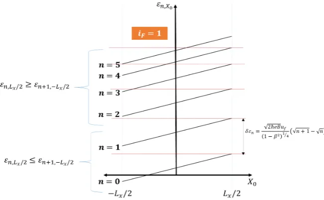
Unlike conventional semiconductors, the energy gap has an E-field depen-dence. As can easily be seen from (1.5), the larger the E-field gets, the larger the energy gap becomes. On the other hand, the larger the L.L. index, the smaller the energy gap. This interplay will play a major role later on, when we consider the thermodynamic occupations of the energy levels. One can always prove that, for a given L.L. index and a value of E-field (such that β<1) there will always be
an unavoidable overlap (states of greater n values have lower energy than states with lower n values). We can set conditions (for arbitrary E and n) for which this kind of overlap is avoided as:
2
, x 1, x 2
n L n L
ε ≤ε+ − (1.6)
To picture this more properly, we provide examples in the graphs shown in
Figure 1.
Condition (1.6) along with (1.4) results in:
(
)
1 4(
)
2
2
1 1
f
x
eBu
n n eEL
β + − ≥
−
or δε ≥n eELx (1.7)
That is, in words, when the work performed by the electric field is smaller than the energy gap at a certain X0, no overlap is observed between the L.L.s n
and n + 1. Generally, for strong enough electric field or for a small enough L.L. index, the above inequality will be true (see Figure 2); but as the L.L. index of occupied levels gets larger (hence for a large number of electrons N) the energy gaps between adjacent L.L.s will become lower, until an inevitable gap closing occurs (Figure 2 providing a concrete example).
We define n=iF to be the topmost L.L., which for a given value of E and B
maintains an energy gap with its adjacent L.L.s: (n= −iF 1, n= +iF 1) Clearly,
L.L. index n= +iF 1 no longer separates from iF +2 with an energy gap, and
in this case, Inequality (1.7) reverses direction: δεiF+1≤eELx. In other words,
L.L.s with n=0,1, 2,,iF do not overlap, while L.L.s with higher quantum
DOI: 10.4236/ampc.2018.81003 35 Advances in Materials Physics and Chemistry
[image:4.595.214.534.77.229.2](a) (b)
Figure 1. (a) An example of an E-field value (strong) that do not cause overlaps between different L.L.s; (b) Another example of a weaker E-field that causes overlaps between ad-jacent L.L.s.
Figure 2. In an arbitrary, fixed E-field strength, overlaps occur as L.L. index gets larger. The overlaps are indicated by the conditions (inequalities) shown at the left of the figure. The red lines indicate the top-most energetic state in a given L.L., in comparison with the next adjacent L.L. lower state. The stronger the E-field gets, the larger the energy gap be-comes, and the overlap will occur at an energetically high L.L. In the above example, overlaps occur between (n = 2, n = 3), (n = 3, n = 4), (n = 4, n = 5, n = 6 (not shown)). Levels n = 0, n = 1 do not overlap and they provide independent energy states when fol-lowing an occupation procedure. In this case, iF=1.
The above is a generic case for an arbitrary value of E and n. Of course there might be cases where overlaps start from n = 0 (for a low enough E-field), in which case iF =0, and all L.L.s with n > 0 overlap. In this case, with no energy
gap present at all, graphene will gain a metallic character. Equation (1.7) with input n= +iF 1 becomes then:
(
)
1 4(
)
2
2
2 1
1
f
F F x
eBu
i i eEL
β + − + ≤
−
[image:4.595.211.537.287.488.2]DOI: 10.4236/ampc.2018.81003 36 Advances in Materials Physics and Chemistry
2. The Strong
E
-Field Regime
After the above discussion and definitions, we proceed to thermodynamic occu-pations of the graphene’s energy levels at zero temperature. For this purpose, we consider a collection of N electrons at T = 0, which fill the lowest energy levels until the Fermi energy denoted by εF. In reality, the Fermi energy is not
con-stant when there is an electric field running through the system; what we then mean by Fermi energy is actually a Fermi point, which is the topmost occupied state in the energy diagram. We also make the supposition that this Fermi point is located on a L.L. indexed with n= −ρ 1 (ρ=1, 2, 3,), so that there are
al-ways ρ L.L.s occupied at any time (the last level n= −ρ 1 being generally
par-tially occupied). First, we will focus on the special case where all ρ Landau Levels are not overlapping, and can be occupied independently by the N electrons. In this case the following relation must be satisfied:
1 iF
ρ − ≤ (2.1)
and for strong enough magnetic fields, it is guaranteed that Equation (2.1) will always be satisfied, and no overlap between L.L.s with different quantum num-bers will be observed. In what follows, we will consider a constant, strong E-field, while the magnetic field may vary, but always in a way that satisfies Equation (2.1).
Considering that the L.L. with n = 0 only has a capacity for 2Φ/Φ0 electrons,
and that all the other n≠0 L.L.s may host up to 4Φ/Φ0 electrons, we find that
in order to have ρ L.L.s occupied, the following inequality must hold:
(
)
(
)
0 0
2 2
2ρ−3 Φ≤N≤ 2ρ−1 Φ
Φ Φ (2.2)
Note that when ρ=1 then
0 2
0≤N≤ Φ
Φ , as N is always a positive number.
Treating N as a constant, we can solve (2.2) with respect to magnetic field B:
(
)
0(
)
01 1
2 2ρ−3 nAΦ ≥ ≥B 2 2ρ−1 nAΦ (2.3)
with nA the electronic surface density and Φ0 the flux quantum. Also note
that we have considered the special case where ρ ≤ +iF 1, where all L.L.s are well
separated with an energy gap, and no inter-L.L. overlapping occurs. (The special case of nonzero overlaps will be considered in the next Section). Note that Equa-tion (2.3) can also describe the well-known unconvenEqua-tional Quantum Hall Effect in graphene, with the Hall conductivity given by the well-known relation:
2 1 4 2 H
A
en e
B h
σ = =ρ−
(2.4)
If one replaces B by the value
(
)
01
2 2 1 A
B n
ρ
= Φ
− ; σH is then quantized in
half-integer multiples of 4e2
h .
DOI: 10.4236/ampc.2018.81003 37 Advances in Materials Physics and Chemistry
= 0) is given as a sum over all states lower than “the Fermi state” or Fermi point, namely
(
)
0
0 , 0 1 4 0
, , 2
2
1
f n X
n X n X
n eBu
E ε eEX
β
= = +
−
∑
∑
(2.5)In the thermodynamic limit Lx→ ∞, we may approximate the sum with
re-spect to X0 as follows:
0 2 0 0 2 4 d x x L y L X BL X − → Φ
∑
∫
for n>0 and0 2 0 0 2 2 d x x L y L X BL X − → Φ
∑
∫
for n=0.(2.6) The total internal energy of the system can then be separated in the energy of the fully occupied bands plus the energy of the partially occupied last L.L. (that contains the Fermi point, n= −ρ 1):
full part
E=E +E (2.7)
In what follows, we will consider the case ρ>1, where the contribution of
the lowest L.L. n = 0 is negligible. Given that all the bands up to n= −ρ 2 are
fully occupied, we may write:
(
)
(
)
2 2
2 2
full 1 0 2 1 4 1 0 0
0 2 0 2
2 1 4 1 2
0
2
4 d 4 d
1 2 4 1 x x x x L L
y f y
L L
i i
f
n
BL n eBu BL eE
E X X X
eBu n ρ ρ ρ β β − − = − = − − = = +
Φ − Φ
Φ = Φ −
∑
∫
∑
∫
∑
(2.8)
To determine Epart, we must first determine the X0 value at the Fermi point
(limit of the X0 integration at the n= −ρ 1 L.L.). From Equation (1.2) we get
for ky =2πl Ly and n= −ρ 1:
(
)
(
)
2
0 2 1 4
2 1 2π 1 B B y l l X l L β ρ β − = −
− (2.9)
The quantum number l, appearing in (2.9) has a starting value l0 that can be
determined by setting 0
2
x
L
X = − as follows:
(
)
(
)
0 1 4
2 0
2 1
2 2π 1
y B L l l β ρ β − Φ = − +
Φ − (2.10)
Now, using the fact that the last L.L. contains
(
)
0 2
2 3
N− ρ− Φ
Φ electrons, we
have all the necessary information to determine the guiding center value of the electron placed at the Fermi point:
(
)
2 0, 0 2π 1 4 F B y N X l L ρ Φ
= − −
Φ
DOI: 10.4236/ampc.2018.81003 38 Advances in Materials Physics and Chemistry
For example, when
(
)
0
2 2 3
N= ρ− Φ
Φ , (meaning that the last L.L. is empty of
electrons), we get from (2.11):
(
) ( )
2 2
0,
0 0
2 2 3
2π π
1 2
4
F B B x
y y
X l l L
L L
ρ
ρ −
Φ Φ
= − − Φ = − = −
Φ
, (2.12)
whereas for
(
)
0
2 2 1
N= ρ− Φ
Φ we have that X0,F =Lx 2, explicitly demonstrating the correctness of our results. The remaining task to carry out is to calculate the energy of the partially occupied L.L. n= −ρ 1
(
)
(
)
(
)
(
)
0, 0,
part 0 2 1 4 0 0
2 2 0 0 2 2 0, 0, 1 4 2 0 0 2 1
4 d 4 d
1
2 1
4 4
2 2 8
1
F F
x x
X f X
y y
L L
f
y x y F x
F
eBu
BL BL
E X eE X X
eBu
BL L BL X L
X eE ρ β ρ β − − − = +
Φ − Φ
−
= + + −
Φ − Φ
∫
∫
(2.13)
Substituting Equation (2.11) into (2.13) we obtain (in units of Fermi energy (in the absence of the electromagnetic field)
ε
F =uF πnA , per particle)(
)
(
)
(
)
[
]
(
)
1 2 3 2
part 1 4 2 0 0 2 0
4 1 2 4 1 2 3
1
1 4 8 3
8 2
F
A A
x
y y A
E B B
N n n
eEBL
NE h eSE
L B L n
ε ρ ρ ρ
β
ρ ρ ρ
= − − − −
Φ Φ
− + − − + − + Φ (2.14)
Finally, adding Equations (2.14) and (2.8) we arrive at the following result:
(
)
[
]
(
)
(
)
(
)
3 2 2
1 4 1
2
0
1 2
2
0 0
4 2 2 3 1
1
4 1 1 4 8 3
8 2
F
n A
x
A y y A
E B
n
N n
eEBL
B NE h eSE
n L B L n
ρ
ε ρ ρ
β
ρ ρ ρ ρ
− = = − − − Φ − + − + − − + − + Φ Φ
∑
(2.15)with 2
1 3 1 2 , 1 2 4π n n
ρ− ζ ρ ζ
= = − − − −
∑
where 1, 12 ζ− ρ−
is the Hurwitz
Zeta function and 3
2 ζ
is the Riemman function. Note the interesting fact
that, terms proportional to electric field strength E result in the following mag-netization:
2 2
0
4 8 3 ,
8 2 x E y A E eEL
M N NE h
N B L B n ρ ρ
∂
= − = − − +
∂ Φ (2.16)
which, when considered at full band occupation (meaning that
(
)
01
2 2 1 A
B n
ρ
= Φ
− )
DOI: 10.4236/ampc.2018.81003 39 Advances in Materials Physics and Chemistry
(
)
22
2 2
0 0
2
4 2 1
4 8 3
8 2
1 2
2 2
H x E
y A A
x x
A A
h eEL
M NE
N L n n
EL e L
E
n h n
ρ
ρ ρ
σ ρ
−
= − − +
Φ Φ
= − =
(2.17)
i.e. the proportional constant is equal to half Hall conductivity, similar to the cor-responding result in a conventional semiconductor case [3]. (Plots of the field-free Energy and Magnetization are given in Figure 3).
3. The Weak
E
-Field Regime
We now proceed to a considerably more difficult case: the low E-field regime. In this regime, as the electric field becomes weaker, the energy gap gets smaller. As a result, there will be an unavoidable point where some L.L.s will overlap (Figure 1(b)), and occupational patterns turn out to be more complex. Inequality (1.7) is no longer true for all n’s (it will indeed be true only for L.L.s with quantum num-ber ≤ iF). If, for simplicity reasons, we suppose for a moment that the energy
spectrum configuration stays the same as before, and that the only change we have is a larger number of electrons N to be placed on the available states, things become a bit clearer. L.L.s up to iF (n=0,1, 2,,iF) won’t overlap with any of
the rest L.L.s, while L.L.s with n=i iF, F+1,iF+2,,ρ−1 will indeed overlap.
In this case, we may also have that ρ − ≥1 iF. Recall from the previous Section
that in addition, the following relation must also hold: β<1.
We fix the Fermi point at n= −ρ 1, with energy given by:
(
)
(
)
1 4 02
2 1
1
f
F F
eBu eEX
ρ ε
β
−
= +
−
(3.1)
with X0F the guiding center position of the last energetically highest electron,
occupying the Fermi point state. For the example case shown in Figure 4, and further supposing that the Fermi point is located at X0F = −Lx 2 (Figure 5)
for simplicity reasons, we have that:
(
2)
1 48
2 1
f x
F
eBu L
eE
ε
β
= −
−
[image:8.595.212.537.526.692.2] (3.2)
DOI: 10.4236/ampc.2018.81003 40 Advances in Materials Physics and Chemistry
Figure 4. Diagram showing the occupations (navy blue) of the lowest energy states up to the Fermi point (red dot). Note that this is the optimal energy configuration for iF=1 and ρ = 5. Landau levels indexed with n = 0 and n = 1 do not overlap, while n = 2 over-laps with n = 3, and n = 3 overlaps with n = 4 and n = 5 (currently not occupied). If the Fermi point were located at i.e.n = 1, meaning that ρ = 2, we would then expect that the Hall conductivity would be quantized according to Equation (2.4). But, now, because of the inclusion of the overlaps, there is no need for an integer quantization, as we shall see in the main text.
[image:9.595.207.536.431.687.2]DOI: 10.4236/ampc.2018.81003 41 Advances in Materials Physics and Chemistry
Now, from the Figure 5, we observe that in this configuration, L.L.s n = 0, 1 and 2 are fully occupied, while L.L. n = 3 is only partially occupied. To deter-mine the exact number of states occupied in L.L. n = 3 we examine its intersec-tion with the Fermi point (red line in Figure 5):
(
2)
1 4 0(
2)
1 46 8
2
1 1
f f x
F
eBu eBu L
eEX eE
β + = β −
− −
(3.3)
which yields for X0F:
(
)
(
)
0 1 4
2 8 6 2 1 f x F eBu L X eE β = − + − −
(3.4)
From the above, we may determine the initial and final values of the kx (that
is, l0 and lf ), namely
(
)
0 1 4
2 0
6
2 2π 1
y B L l l β β Φ = − +
Φ − (3.5)
(
)
1 4(
)
(
)
1 42 2
0
6
8 6
2 1 1
y F y
f
F
BL eBu EL e
l
Eh β hu eB β
Φ
= − + − +
Φ − −
(3.6)
The number of states in L.L. n = 3 is then given by the difference of the initial and final values of l, namely
(
)
(
)
0 2 1 4 8 6
1 y F f BL eBu l l Eh β − = − −
(3.7)
and the total number of states below the Fermi point reads:
(
2)
1 4(
)
0 0 0 1,2
2 8 6
1 y F n n BL eBu g Eh β = = Φ Φ = + + −
Φ Φ −
(3.8)
Because all these states are filled with electrons (4 electrons in each state for n > 0 and 2 electrons for n = 0) we have that:
(
)
(
)
(
)
(
)
1 4 2 0 0 1 4 2 02 8 4 8 6
1
10 4 8 6
1 y F y F BL eBu N Eh BL eBu Eh β β Φ Φ = + + −
Φ Φ −
Φ
= + −
Φ −
(3.9)
Equation (3.9) yields for the Hall conductivity:
(
)
(
)
2
1 4 2
10 4 8 6
1
y F
H
A eL
en e eBu
B h SEh
σ
β
= = + −
−
(3.10)
forma-DOI: 10.4236/ampc.2018.81003 42 Advances in Materials Physics and Chemistry
tion of localized and extended states that lie inside this gap. When the gap is de-stroyed, the system becomes metallic; it may thus not be unreasonable to find a Hall conductivity that is electric/magnetic field-dependent, destroying the pla-teaux formation. This is something that needs to be further investigated experi-mentally.
4. Conclusion
In this work, a thermodynamic study has been conducted with respect to a 2D Graphene monolayer subjected to crossed electric and magnetic fields. Thermo-dynamic quantities like the global energy and magnetization have been exactly and analytically determined, in combination with transport properties, i.e. the Hall conductivity. The results suggest exotic possibilities that are here pointed out as a natural outcome of an exact and careful calculation in the noninteracting elec-trons many-body framework, and these necessitate exceedingly careful experimental investigation. Finally, with respect to the range of validity, although our results in-volve no approximations whatsoever, the general role of disorder in combination with the above physics of the strong fields is certainly something that needs fur-ther study.
References
[1] Franz, M. and Molenkamp, L., Eds. (2013) Contemporary Concepts of Condensed Matter Science. Volume 6. Topological Insulators. Elsevier, Amsterdam.
[2] Hideo Aoki, S. and Dresselhaus, M., Eds. (2014) Physics of Graphene. Springer, Berlin. https://doi.org/10.1007/978-3-319-02633-6
[3] Takahashi, R. (2015) Topological States on Interfaces Protected by Symmetry. Chapter 4: Weyl Semimetal in a Thin Topological Insulator. Springer, Berlin. https://doi.org/10.1007/978-4-431-55534-6
[4] Prange, R.E. and Girvin, S.M. (1990) The Quantum Hall Effect. Springer, Berlin. https://doi.org/10.1007/978-1-4612-3350-3
[5] Yoshioka, D. (2002) The Quantum Hall Effect. Springer, Berlin. https://doi.org/10.1007/978-3-662-05016-3
[6] Konstantinou, G. and Moulopoulos, K. (2017) Ground State Thermodynamic and Response Properties of Electron Gas in a Strong Magnetic and Electric Field: Exact Analytical Solutions for a Conventional Semiconductor and for Graphene. Journal of Applied Mathematics and Physics, 5, Article ID: 74872.
https://doi.org/10.4236/jamp.2017.53055
[7] Lukose, V., Shankar, R. and Baskaran, G. (2007) Novel Electric Field Effects on Landau Levels in Graphene. Physical Review Letters, 98, Article ID: 116802. https://doi.org/10.1103/PhysRevLett.98.116802
[8] Kawaji, S., Hirakawa, K. and Nagata, M. (1993) Device-Width Dependence of Pla-teau Width in Quantum Hall States. Physica B: Condensed Matte, 184, 17. https://doi.org/10.1016/0921-4526(93)90313-U
DOI: 10.4236/ampc.2018.81003 43 Advances in Materials Physics and Chemistry Heterostructures under Non-Ohmic Conditions. Journal of Physics C, 16, 5441. https://doi.org/10.1088/0022-3719/16/28/012
[11] Lilly, M.P., Cooper, K.B., Eisenstein, J.P., Pfeiffer, L.N. and West, K.W. (1999) Evi-dence of an Anisotropic State of Two-Dimensional Electrons in High Landau Le-vels. Physical Review Letters, 82, 394-397.
https://doi.org/10.1103/PhysRevLett.82.394
[12] Kazarinov, R.F. and Luryi, S. (1982) Quantum Percolation and Quantization of Hall Resistance in Two-Dimensional Electron Gas. Physical Review B, 25, 7626-7630. https://doi.org/10.1103/PhysRevB.25.7626
[13] Tsemekhman, V., et al. (1997) Theory of the Breakdown of the Quantum Hall Ef-fect. Physical Review B, 55, R10201.https://doi.org/10.1103/PhysRevB.55.R10201 [14] Kramer, T. (2006) Landau Level Broadening without Disorder, Non-Integer
Pla-teaus without Interactions—An Alternative Model of the Quantum Hall Effect. Re-vista Mexicana de Fisica, 52, 49-55.
[15] Peres, N.M.R. and Castro, E.V. (2007) Algebraic Solution of a Graphene Layer in a Transverse Electric and Perpendicular Magnetic Fields. Journal of Physics: Con-densed Matter, 19, Article ID: 406231.