Solving Stiff Reaction Diffusion Equations Using Exponential Time Differences Methods

(1)

http://www.scirp.org/journal/ajcm ISSN Online: 2161-1211 ISSN Print: 2161-1203

DOI: 10.4236/ajcm.2018.81005 Mar. 16, 2018 55 American Journal of Computational Mathematics

Solving Stiff Reaction-Diffusion Equations Using

Exponential Time Differences Methods

H. A. Ashi

The Mathematical Department, King AbdulAziz University, Jeddah, KSA

Abstract

Reaction-diffusion equations modeling Predator-Prey interaction are of cur-rent interest. Standard approaches such as first-order (in time) finite differ-ence schemes for approximating the solution are widely spread. Though, this paper shows that recent advance methods can be more favored. In this work, we have incorporated, throughout numerical comparison experiments, spec-tral methods, for the space discretization, in conjunction with second and fourth-order time integrating methods for approximating the solution of the reaction-diffusion differential equations. The results have revealed that these methods have advantages over the conventional methods, some of which to mention are: the ease of implementation, accuracy and CPU time.

Keywords

Finite Difference Methods, Exponential Integrator, Exponential Time Differencing Method, Reaction-Diffusion System

1. Introduction

Numerical methods are important tools in investigating the solution’s behavior of non-linear realistic models in biology [1] where no closed form solutions exist. A class of these models is reaction diffusion (RD) problems that, for instant, reproduce some of the complex pattern observed on the skin of certain animals. This includes the development of coat patterns on mammals and the patterning of butterfly wings [1].

Reaction diffusion models have been studied extensively since the RD theory first proposed by Turing [2] to describe the range of spatial patterns observed in the developing embryo.

In recent years, several theoretical models, regarding spatial pattern, have How to cite this paper: Ashi, H.A. (2018)

Solving Stiff Reaction-Diffusion Equations Using Exponential Time Differences Me-thods. American Journal of Computational Mathematics, 8, 55-67.

https://doi.org/10.4236/ajcm.2018.81005

Received: December 28, 2017 Accepted: March 13, 2018 Published: March 16, 2018

http://creativecommons.org/licenses/by/4.0/

(2)

DOI: 10.4236/ajcm.2018.81005 56 American Journal of Computational Mathematics

been introduced and led to a better understanding of how these patterns arise from certain mechanism. A general theoretical framework for studying pattern formation in biological systems within a growing domain was developed in [3]. In addition, reaction diffusion equations modeling predator-prey interactions have been paid attention and studied extensively [4][5][6]. In these models, the most important element is the “ functional response”, the function that describes the number of prey consumed by predator per unit time.

For the numerical solution of nonlinear reaction diffusion problems (most of which are stiff1_{), fully explicit temporal methods are avoided due to the sever}

restriction on the time step size imposed by the stiff diffusion term. Fully implicit temporal schemes are not recommended since they have the task of solving large implicit systems at each time step. Alternatively, several methods were introduced. The vast majority of scientific community uses, for the spatial discretization, lower-order centred finite differences schemes due to the ease of implementation and incorporation of the boundary conditions in a straightforward way. The time integration is carried out, usually, by using some types of low-order time step methods such as, second-order fully implicit Crank-Nicholson methods.

The Exponential Time Differencing (ETD) methods [12] in conjunction with spectral methods [13] [14] [15] have emerged as viable alternatives to classical schemes for a wide variety of problems. Their applications to solve reaction-diffusion problems [6][16] [17][18][19] have been steadily growing. Spectral methods are popular for generating spectral accurate spatial derivatives, through built-in codes in Matlab [20]. ETD schemes recover the exact solution to the linear part (which is generally the most stiff part of the system), and integrate exactly an approximation of the non-linear terms. We may approximate the non-linear parts by some polynomial in time that may be calculated using previous steps of the integration process (producing multi-step ETD methods) or by Runge-Kutta-like stages (resulting in ETD schemes of RK type), see [21] for a comprehensive review. The numerical computation of the ETD coefficients, which are functions related to the matrix exponential, arises some difficulties [22] [23]. Fortunately, several numerical algorithms [19][22]-[28] were introduced to enhance the accuracy in computing these coefficients.

The work presented in this article is motivated by the theoretical and computational study by Gavie [5] for the dynamical properties of the 2-component reaction-diffusion system modeling predator-prey interactions with the Holling type II functional response. The system displays a wide spectrum of ecologically relevant behavior, including chaos. The model and an illustration of the computational study conducted by Garvie [5], using first-order finite difference

1_{Stiff differential equations are categorized as those whose solutions (or different components of a}

(3)

schemes, are briefly described in §2. In §3, we numerically approximate the solution of the predator-prey model in two dimensions employing spectral methods, for the space discretization, in conjunction with high-order time integrating methods. The results of the numerical experiment are compared to Garvie’s findings. Section §4 recaps our results and points out some conclusions.

2. Model Problems

In this section we briefly give the 2-component reaction-diffusion non-dimensional system, modeling predator-prey interactions with the Holling type II functional response and logistic growth of the prey, as follows (taken from [5]):

(

)

( )

1 ,

.

u

u u u vh au

t v

v bvh au cv

t δ

∂

= ∆ + − −

∂ ∂

= ∆ + −

∂

(1)

The population densities of the prey and predators at time t and vector position x are denoted by u

( )

x,t and v

( )

x,t respectively. ∆ is the usual

Laplace operator in d≤3 space dimensions and the parameters a b c, , and

δ are strictly positive. The domain (habitat), defined by Ω_{, is bounded and} configured with appropriate initial condition and zero-flux boundary conditions, ensuring that no individual species can leave the domain. The “functional response” h

( )

⋅ represents the prey consumption rate per predator as a fraction

of the maximal consumption rate. It is assumed to be a 2

C function satisfying

the following conditions: • h

( )

0 =0,

• lim

( )

1

x→∞h x = ,

• h

( )

⋅ is strictly increasing on

[

0,∞

)

.

A specific type II functional response with positive parameters α β, and γ

is given as follows [5]

( )

,

(

)

, with 1 , , .

1

h η η η au a α b β c γ

η

= = = = =

+

Thus, the type of kinetics governed in this paper is

( ) (

, 1

)

uv , ,

( )

uv .

f u v u u g u v v

u u

β

_γ

α

= − − = −

+ + (2)

We consider the natural biological meaningful region u≥0, 0v≥ with

(4)

Computational Issues

For the two dimensional approximation, let n=1,,N and i j, =0,,J,

where N and J denote the number of uniform subdivision of the time interval

[ ]

0,T and the square domain Ω =

[

A B,

] [

× A B,

]

, 0A<B respectively. The

forward difference in time and the five point central difference approximation of the Laplace in two dimensions are defined as follows:

(

)

(

)

1

2

, , 1 , 1 1, 1, ,

,

4 ,

n n n

n

h i j i j i j i j i j i j

U U U t

U U U U U U h

−

+ − + −

∂ = − ∆

∆ = + + + −

where ∆ =t T N and h=

(

B−A

)

J represent the time and space step

respectively. In addition, suppose that ,

n i j

U and ,

n i j

V denote the two dimensional

approximation to the solutions u and v respectively at the point

(

x y ti, j, n

)

, where the time levels tn = ∆n t.

Garvie [5] presents two first-order semi-implicit (in time) finite difference schemes as follows:

1 , , 1

, , , , , 1

, 1

, ,

, , 1 ,

,

.

n n i j i j

n n n n n

n i j h i j i j i j i j n i j n n

i j i j

n n n

n i j h i j n i j i j

V U

U U U U U

U

V U

V V V

U α β δ γ α − − − − − ∂ = ∆ + − − + ∂ = ∆ + − + (3) 1 1 , ,

1 1 1

, , , , , 1

, 1 1

, , 1

, , 1 ,

,

n n i j i j

n n n n n

n i j h i j i j i j i j n i j n n

i j i j

n n n

n i j h i j n i j

i j

V U

U U U U U

U

V U

V V V

U α β δ γ α − − − − − − − − − − ∂ = ∆ + − − + ∂ = ∆ + − + (4)

with the given initial approximations

(

)

(

)

0 0

, 0 , , , 0 , ,

i j i j i j i j

U =u x y V =v x y

and zero-flux boundary conditions, for studying the dynamics of spatially extended predator-prey interaction with logistic growth of the prey (1) in two space dimensions. The “analytical solution” of the predator-prey system (1) is approximated using schemes (3) and (4) on a fine mesh and small time step. The linear system of algebraic equations, resulting from the solution of the problem using either schemes, is sparse, banded and has a simple structure (tridiagonal and block tridiagonal system in one and two dimensions respectively). In addition, the coefficient matrices of the linear system are strictly diagonally dominant, which guarantee the convergence of the GMRES algorithm (an iterative solver) used to solve the system (in two dimensions), see [5].

The convergence of Schemes (3) and (4) was decided on upon reducing the time step until the difference between the approximations from either schemes is negligible. On the other hand, the space step is kept sufficiently small to see clearly the qualitative feature of the solutions.

(5)

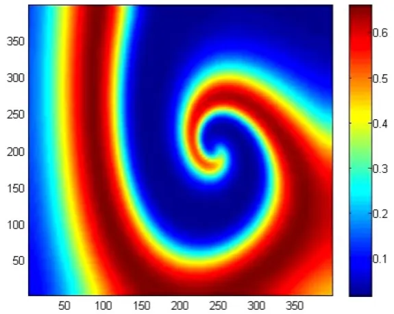
DOI: 10.4236/ajcm.2018.81005 59 American Journal of Computational Mathematics • For various initial conditions, the evolution of the system led to the formulation of spiral patterns, see Figure 1, followed by irregular patches covering the whole domain (spatio-temporal chaos).

• Schemes (3) and (4) are simple to program, stable and convergent provided that the time step is below a (non-restrictive) critical value.

• The disadvantage of the code is that the run time can be prohibitive when using a combination of large domain size and final time T coupled with small space and time step.

From an ecological point of view, Garvie stated that in the absence of external influences, certain initial conditions can lead to spatial and temporal variants in the densities of predator and prey that persist indefinitely.

The section following gives an overview of higher-order competing methods: Exponential Time Differencing (ETD) methods §3.1, Integrating Factor (IF) methods §3.2 and Implicit-Explicit methods (IMEX) §3.3 utilized for simulating the numerical solution of the prey-predator system (1) with kinetics (2) in two dimensions.

3. Numerical Experiments

[image:5.595.229.517.404.633.2]

We numerically compare the performance of the first-order (in time) schemes (3) and (4), outlined in §2.1, with that of the second and fourth-order time integrating methods including: Exponential Time Differencing (ETD) methods

Figure 1. The approximated prey densities , n i j

U for kinetics (2) in two dimensions at

150

T = . The initial conditions are given by

(

)(

)

0 7

, 6 35 2 10 0.1 225 0.1 675

i j i j i j

U = − × − x − y − x − y − ,

(

)

(

)

0 5 4

, 116 245 3 10 450 1.2 10 150

i j i j

V = − × − x − − × − y − with α =0.4, β =2.0,

0.6

(6)

§3.1, Integrating Factor (IF) methods §3.2 and Implicit-Explicit methods (IMEX) §3.3, for approximating the solution of the prey-predator system (1) with kinetics (2) in two dimensions. The aim is to observe the effectiveness of the competing methods, taking into account the accuracy and CPU time consumed by the methods.

3.1. Exponential Time Differencing Methods

Consider for simplicity a single model of a stiff ordinary DE

( )

_{( )}

₍

_{( )}

₎

d

, ,

d u t

cu t F u t t

t = + (5)

where c is the stiffness parameter and F u t t

(

( )

,

)

is the non-linear forcing term,

then the first-order ETD1 scheme [12][29] is

(

)

1 e e 1 ,

c t c t

n n n

u + =u ∆ + ∆ − F c

where ∆t is the time step and u_n and Fn denote the numerical approximation to u t

( )

n and F u t

(

( )

n ,tn

)

respectively.

The second-order ETD Runge-Kutta method ETD2RK1 [12] analogous to the “improved Euler” is

(

)

(

)

(

)

( )

2

1

e e 1 ,

e 1 , ,

c t c t

n n n

c t

n n n n n

a u F c

u a c t F a t t F c t

∆ ∆

∆ +

= + −

= + − ∆ − + ∆ − ∆ (6)

where term an approximates the value of u at tn+ ∆t. Also, the ETD2RK2 scheme [23] analogous to the “modified Euler” method is

(

)

(

)

(

)

{

(

)

(

)

}

2 2 1 2

e e 1 ,

e 2 e 2

2 e 1 , 2 .

c t c t

n n n

c t c t

n n n

c t

n n

a u F c

u u c t c t F

c t F a t t c t

∆ ∆ ∆ ∆ + ∆ = + − = + ∆ − + ∆ + + − ∆ − + ∆ ∆ (7)

A fourth-order scheme ETD4RK [12] is obtained as follows:

(

)

(

)

(

)

(

)

(

)

2 2 2 2 2 2

e e 1 ,

e e 1 , 2 ,

e e 1 2 , 2 ,

c t c t

n n n

c t c t

n n n n

c t c t

n n n n n

a u F c

b u F a t t c

c a F b t t F c

∆ ∆ ∆ ∆ ∆ ∆ = + − = + − + ∆ = + − + ∆ −

(

)

(

)

{

(

)

(

)

(

)

(

)

(

)

(

)

(

)

}

(

)

2 2 1

2 2 3 2

e 3 4 e 4

2 2 e 2 , 2 , 2

4 e 3 4 , .

c t c t

n n n

c t

n n n n

c t

n n

u u c t c t c t F

c t c t F a t t F b t t

c t c t c t F c t t c t

∆ ∆ + ∆ ∆ = + ∆ − ∆ + − ∆ − + ∆ − + ∆ + + ∆ + + ∆ + − ∆ + − ∆ − ∆ − + ∆ ∆ (8)

The terms an and bn approximate the values of u at tn+ ∆t 2 and the term cn approximates the value of u at tn+ ∆t.

3.2. Integrating Factor Methods

(7)

(

)

1 e .

c t

n n n

u+ = u + ∆tF ∆

The second-order Integrating Factor Runge-Kutta (IFRK2) method [12] is given by

(

)

(

)

(

)

1 e ,

e , , 1 e , 2 c t n n c t

n n n n

c t

n n n n

a tF

b tF u tF t t

u u a b

∆ ∆ ∆ + = ∆ = ∆ + ∆ + ∆ = + + (9)

and the Integrating Factor Runge-Kutta (IFRK4) method [25][30][31] is

(

)

(

)

(

)

(

)

(

)

(

)

2 /2 2 2 1 ,

2 e , 2 , 2 , 2 , e e , 2 ,

1

e e 2 e .

6

n n

c t

n n n n

c t

n n n n

c t c t

n n n n

c t c t c t

n n n n n n

a tF

b tF u a t t

c tF u e b t t

d tF u c t t

u u a b c d

∆ ∆ ∆ ∆ ∆ ∆ ∆ + = ∆ = ∆ + + ∆ = ∆ + + ∆ = ∆ + + ∆ = + + + + (10)

3.3. Implicit-Explicit Methods (IMEX)

The usefulness of the IMEX schemes is apparent when it is coupled with spectral methods, for approximating spatially discretized reaction-diffusion problems [32] arising in chemistry and mathematical biology. The most popular method is the second-order linear-multi-step IMEX scheme (AB2AM2) [33]

(

)

1 1 3 1 .

2

n n n n n n

t

u₊ =u +∆ _c u +u₊ + F −F₋ _ (11)

For the time discretization, this method treats the non-linear reaction term explicitly utilizing the second-order Adams-Moulton methods, while the diffusion term is treated implicitly utilizing the second-order Adams-Bashforth schemes.

IMEX methods are restricted from having an order higher than two if A-stability is required. Therefore, despite their simplicity and frequent usage, they are not extendable to higher order.

3.4. Comparison Experiments and Results

The overall efficiency of the methods in our numerical experiments is measured by three dominant testing parameters: the accuracy, the start-up overhead cost and the CPU time consumed by the methods. All the calculations presented in this paper are performed using Matlab codes.

For the simulation tests, we choose Neumann boundary conditions

(

)

(

)

(

)

(

)

, , , ,

0 , 0 400,

, , , ,

0 , 0 400,

u x y t v x y t

x

x x

u x y t v x y t

(8)

and apply discrete Fourier cosine series approximation for the spatial discretization using NF_x =NF_y =256 grid spatial points. The spatial grids are

set to be fine enough such that the errors are dominated by those from the time integration. We can write the test model problem (1) in Fourier space, taking the advantage of the 2-dimensional discrete cosine transform routine dct2 built in

Matlab as follows:

( )

₍

₎

_{( )}

₍

_{( )}

₎

( ) ( )

( )

₍

₎

_{( )}

( ) ( )

( )

2 2

ˆ d

ˆ 1 ,

d

ˆ d

ˆ ,

d

k

x y k

k

x y k

u t u t v t

k k u t u t u t

t u t

v t u t v t

k k v t v

t u t

α β

γ α

 

= − + + _ − − _

+

 

 

= − + + _ − _

+

 

dct2

(12)

where α =0.4, 2, 0.6, 1β= γ = δ = and k kx, y represent the wave-numbers in two dimensions. The linear (diffusion) operator in the resulting uncoupled system of ordinary differential equations (ODEs) (12) is diagonal, with elements

(

2 2

)

x y

k k

− + , of which some has large negative real eigenvalues that represent decay on a time scale much shorter than that typical of the non-linear term (strong dissipation dynamics), causing system (12) to be stiff. The non-linear term is transformed to physical space and evaluated at the uniform grid points and then transformed back to spectral space.

Afterword, we integrate the system of ODEs (12) in time up to t=150

employing second and fourth-order stiff integrators including: Exponential Time differencing ETD2RK1(6), ETD2RK2 (7), ETD4RK (8) methods, Integrating Factor IFRK2 (9), IFRK4 (10) methods and a second-order Implicit-Explicit AB2AM2 (11) method. We focus on the initial approximation (taken from [5]) given by

(

)(

)

0 7

, 6 35 2 10 0.1 225 0.1 675 ,

i j i j i j

U = − × − x − y − x − y −

(

)

(

)

0 5 4

, 116 245 3 10 450 1.2 10 150 .

i j i j

V = − × − x − − × − y −

Considering the implementation of the above time discretization methods, we evaluate three coefficients2_{for the ETD2RK1(6), the ETD2RK2 (7) methods and}

four coefficients for the ETD4RK (8) method, once at the beginning of the integration for each value of the time-step sizes, by means of contour integra-tion3_{in the complex plane approximated by the Trapezium rule. We choose}

circular contours, each is centred at one of the elements that are on the diagonal matrix of the linear part of the semi-discretized model (12), with radius R=1

and sampled at 32 equally spaced points. Moreover, in the main loop of integration, the ETD2RK1, the ETD2RK2, the IFRK2 (9), the ETD4RK and the IFRK4 (10) methods perform two (for the second-order methods) and four (for the fourth-order methods) function transforms per time step. The IF schemes require, in addition, the evaluation of one or more matrix exponentials, for

2_{The ETD-RK methods require an accurate algorithm for evaluating the coefficients of}

(

( )

_,

)

n n

F u t t

to avoid numerical difficulties, see [22][23].

3_{The “Cauchy integral” approach was proposed by Kassam and Trefethen, see}_[25]_[31]_{for further}

(9)

which acceptable algorithms are well known [29][34].

In our tests, we measure the accuracy of the methods in terms of the relative error evaluated in the integrated error norm. The numerical “exact” solution is approximated on a fine mesh with a very small time-step size and compared with the corresponding approximated solution with a sequence of large time steps.

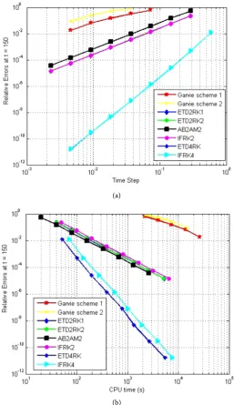
Figure 2(a) summarizes the temporal accuracy behavior for all the methods

(a)

[image:9.595.244.502.192.638.2]

(b)

Figure 2. Relative errors versus (a) time step (b) CPU time for the prey-predator system (1) with kinetics (2) in two dimensions. The initial conditions are given by

(

)(

)

0 7

, 6 35 2 10 0.1 225 0.1 675

i j i j i j

U = − × − x − y − x − y − ,

(

)

(

)

0 5 4

, 116 245 3 10 450 1.2 10 150

i j i j

V = − × − x − − × − y − with α =0.4, β =2.0,

0.6

(10)

and confirms the expected order for all of them. In the figure, we plot the numerical relative error of the integrated error norm as a function of the time step. The time-step values are selected to ensure that all methods achieve stable accurate results. The plot indicates, firstly, that the fourth-order methods take the largest time-step size, i.e. the fewest number of steps, to converge to a solution within a fixed given relative error in the figure. On the other hand, the first-order schemes (3) and (4) break down (errors are of O

( )

1 ) for time-step

size larger than 4

2

t −

∆ ≈ _{because of the numerical stability constraints.} Secondly, a fixed reduction in the time-step size will produce a greater reduction in the error for the second and fourth order methods than for the first-order schemes (3) and (4).

For an additional preference between the methods compared, we valued the accuracy with respect to the CPU time, illustrated in Figure 2(b). For the first-order schemes (3) and (4), the computation cost is almost identical, per time step.

Second-order convergence is confirmed in Figure 2(a) for the ETD2RK1(6), the ETD2RK2 (7), the AB2AM2 (11) and the IFRK2 (9) methods. All second-order methods successfully integrate the system for time-step sizes 2

2

t −

∆ ≈ _{and less.} In addition, the corresponding errors for all methods (except for that of the AB2AM2 method which is considered to be the least accurate) lie approximately on the same line for all values of the time-step. Regarding the CPU time, Figure 2(b) indicates that the variation in time consumption for all methods, for a given level of accuracy, is insignificant.

For the fourth-order methods, the performance of the IFRK4 (10) method resembles that of the ETD4RK (8) method, and the errors are identical and all scale with the expected

( )

4

t

∆ order, see Figure 2(a). However, according to Figure 2(b), the IFRK4 method uses a slightly longer computation time than the ETD4RK method for a given error tolerance.

Clearly the fourth-order methods have a superior performance, as the accuracy and speed are improved significantly compared to lower order methods referring to Figure 2(a) and Figure 2(b) respectively. The fourth order methods have the advantages of gaining order of magnitude of accuracy, even for larger time steps 1

2

t −

∆ ≈ _{, greater than lower order methods.}

In general, we find that out of all comparable methods, the fourth-order methods are the most accurate, for a given time-step size, and the least time consuming for a given level of accuracy, see Figure 2(a) and Figure 2(b) respectively. However, the ETD4RK method was found to be the best scheme for providing accurate stable solution in a fast and efficient way. On the other hand, the most expensive with high computational cost and unpleasant performance are schemes (3) and (4). Thus, the greater accuracy of the ETD4RK and the IFRK4 methods rewards the extra programming efforts.

4. Conclusions

(11)

problems, a simple first-order semi-implicit scheme is the first choice [5] due to the difficulties introduced by the combination of non-linearity and stiffness of a PDE, the complexity both of analysis and implementation of higher order methods, and the increased computer storage required by these methods. However, in tow and higher space dimensions problems, simulations based upon the more conventional ideas become more time consuming. Higher order time integration methods can result in significant benefits in run time reduction while maintaining high accuracy.

In this paper, spectral methods, coupled with second and fourth order exponential integrator methods, are used for solving a reaction-diffusion problem modeling predator-prey interaction. The spectral methods offer several advantages over finite-difference methods such as, accurate discretization of spatial derivatives, ease of implementation and applicability to a wide varies of equations [23][25] [31].

Exponential time stepping solvers are used to remove the the stiffness associated with the diffusive terms, and hence, the severe restriction on the time-step for reasons of stability, allowing much larger time-steps to be selected and the selection is only limited by accuracy.

In our comparison experiment, we have shown that the fourth-order ETD4RK (8) and IFRK4 (10) methods have aided the simulation of model (1) in tow dimensions with improvements of the computational efficiency and speed over first and second-order methods.

Although we focus on system (1) in this paper, we believe that the numerical methods described here and our results can also be extended with modification to numerically solve other non-liner wave problems, models which include advection and reaction-diffusion-convection systems.

References

[1] Murray, J.D. (1993) Mathematical Biology. 2nd Edition, Springer-Verlag, Berlin Heidelberg.

[2] Turing, A. (1952) The Chemical Basis of Morphogenesis. Philosophical Transac-tions of the Royal Society B, 237, 37-72. https://doi.org/10.1098/rstb.1952.0012 [3] Neville, A.A., Matthews, P.C. and Byrne, H.M. (2006) Interactions between Pattern

Formation and Domain Growth. Bulletin of Mathematical Biology, 68, 1975-2003. https://doi.org/10.1007/s11538-006-9060-5

[4] Haque, M. (2009) Ratio-Dependent Predator-Prey Models of Interacting Popula-tions. Bulletin of Mathematical Biology, 71, 430-452.

https://doi.org/10.1007/s11538-008-9368-4

[5] Garvie, M.R. (2007) Finite-Diﬀerence Schemes for Reaction-Diﬀusion Equations Modelling Predator-Prey Interactions in MATLAB. Bulletin of Mathematical Biol-ogy, 69, 931-956. https://doi.org/10.1007/s11538-006-9062-3

[6] Apreutesei, N. and Dimitriu, G. (2010) On a Preypredator Reactiondiﬀusion System with Holling Type III Functional Response. Journal of Computational and Applied Mathematics, 235, 366-379. https://doi.org/10.1016/j.cam.2010.05.040

(12)

Annual Review of Biophysics and Bioengineering, 6, 525-542. https://doi.org/10.1146/annurev.bb.06.060177.002521

[8] Hairer, E. and Wanner, G. (1996) Solving Ordinary Diﬀerential Equations II. 2nd Edition, Springer-Verlag, Berlin. https://doi.org/10.1007/978-3-642-05221-7 [9] Shampine, L.F. and Gear, C.W. (1979) A User’s View of Solving Stiﬀ Ordinary

Diﬀerential Equations. SIAM Review, 21, 1-17. https://doi.org/10.1137/1021001 [10] Gear, C.W. (1971) Automatic Integration of Ordinary Diﬀerential Equations.

Com-munications of the ACM, 14, 176-179. https://doi.org/10.1145/362566.362571 [11] Curtiss, C.F. and Hirschfelder, J.O. (1952) Integration of Stiff Equations.

Proceed-ings of the National Academy of Sciences, 38, 235-243. https://doi.org/10.1073/pnas.38.3.235

[12] Cox, S.M. and Matthews, P.C. (2002) Exponential Time Differencing for Stiff Sys-tems. Journal of Computational Physics, 176, 430-455.

https://doi.org/10.1006/jcph.2002.6995

[13] Boyd, J.P. (2001) Chebyshev and Fourier Spectral Methods. 2nd Edition, Dover, New York.

[14] Fornberg, B. (1996) A Practical Guide to Pseudo-Spectral Methods. Cambridge University Press, Cambridge. https://doi.org/10.1017/CBO9780511626357

[15] Fornberg, B. and Driscoll, T.A. (1999) A Fast Spectral Algorithm for Nonlinear Wave Equations with Linear Dispersion. Journal of Computational Physics, 155, 456-467. https://doi.org/10.1006/jcph.1999.6351

[16] Craster, R.V. and Sassi, R. (2006) Spectral Algorithm for Reaction-Diffusion Equa-tions. Note del Polo 99, Universita degli Studi di Milano, Polp Didattico e di Ricerca di Crema.

[17] Dimitriu, G. and Tefanescu, R.S. (2009) Numerical Experiments for Reaction-Diffusion Equations Using Exponential Integrators. N. A. A., 5434, 249-256.

https://doi.org/10.1007/978-3-642-00464-3_26

[18] Kassam, A.K. (2003) Solving Reaction-Diffusion Equations 10 Times Faster. Oxford University, Oxford, Numerical Analysis Group Research Report No. 16.

[19] Khaliq, A.Q.M., Martin-Vaquero, J., Wade, B.A. and Yousuf, M. (2009) Smoothing Schemes for Reaction-Diffusion Systems with Nonsmooth Data. Journal of Com-putational and Applied Mathematics, 223, 374-386.

https://doi.org/10.1016/j.cam.2008.01.017

[20] Trefethen, L.N. (2000) Spectral Methods in MATLAB. SIAM, Philadelphia. https://doi.org/10.1137/1.9780898719598

[21] Minchev, B.V. and Wright, W.M. (2005) A Review of Exponential Integrators for First Order Semi-Linear Problems. Tech. Rep. NTNU.

[22] Ashi, H.A., Cummings, L.J. and Matthews, P.C. (2009) Comparison of Methods for Evaluating Functions of a Matrix Exponential. Applied Numerical Mathematics, 59, 468-486. https://doi.org/10.1016/j.apnum.2008.03.039

[23] Ashi, H.A. (2008) Numerical Methods for Stiff Systems. PhD Thesis, University of Nottingham, Nottingham.

[24] Skaflestad, B. and Wright, W.M. (2009) The Scaling and Modified Squaring Method for Matrix Functions Related to the Exponential. Applied Numerical Mathematics, 59, 783-799. https://doi.org/10.1016/j.apnum.2008.03.035

(13)

DOI: 10.4236/ajcm.2018.81005 67 American Journal of Computational Mathematics [26] Schmelzer, T. and Trefethen, L.N. (2007) Evaluating Matrix Functions for Ex-ponential Integrators via Carathéodory-Fejér Approximation and Contour Inte-grals. Electronic Transactions on Numerical Analysis, 29, 1-18.

[27] Higham, N.J. (2005) The Scaling and Squaring Method for the Matrix Exponentials Revisited. SIAM Journal on Matrix Analysis and Applications, 26, 1179-1193. https://doi.org/10.1137/04061101X

[28] Koikari, S. (2007) An Error Analysis of the Modified Scaling and Squaring Method. Computers & Mathematics with Applications, 53, 1293-1305.

https://doi.org/10.1016/j.camwa.2006.04.032

[29] Beylkin, G., Keiser, J.M. and Vozovoi, L. (1998) A New Class of Time Discretization Schemes for the Solution of Nonlinear PDEs. Journal of Computational Physics, 147, 362-387. https://doi.org/10.1006/jcph.1998.6093

[30] Berland, H., Skeflestad, B. and Wright, W.M. (2007) EXPINT—A Matlab Package for Exponential Integrators. ACM Transactions on Mathematical Software, 33, Ar-ticle No. 4.

[31] Kassam, A.K. and Trefethen, L.N. (2005) Fourth-Order Time Stepping for Stiff PDEs.SIAM: SIAM Journal on Scientific Computing, 26, 1214-1233.

https://doi.org/10.1137/S1064827502410633

[32] Ruuth, S.J. (1995) Implicit-Explicit Methods for reaction-Diffusion Problems in Pattern Formation. Journal of Mathematical Biology, 34, 148-176.

https://doi.org/10.1007/BF00178771

[33] Ascher, U.M., Ruuth, S.J. and Wetton, B.T. (1995) Implicit-Explicit Methods for Time-Dependent Partial Differential Equations. SIAM Journal on Numerical Anal-ysis, 32, 797-823.

[34] Moler, C. and Van Loan, C. (2003) Nineteen Dubious Ways to Compute the Expo-nential of a Matrix, Twenty-Five Years Later. SIAM Review, 45, 3-49.