Maintenance Strategy Selection for Several
Components of LD-Converter - A Case Study
Subash Kumar Jaladhi1, Dr. M. Murali Krishna2, TNV. Ashok Kumar3, MVS Pavan Kumar4
1
Assistant professor, Dept. of Mechanical Engineering, Sasi Institute of Technology & Engineering, Tadepalligudem
2
Principal, Visakha Technical Campus, Visakhapatnam.
3, 4
Assistant professor, Dept. of Mechanical Engineering, Sasi Institute of technology & Engineering, Tadepalligudem
Abstract: This work is aimed to derive a suitable maintenance strategy for components of LD Converter in steel melting shop. Selection of appropriate maintenance strategy is viability to good economic advantage of manufacturing industries. The study discusses and presents the combined Analytic Hierarchy Process (AHP) – Goal Programming (GP) methodology in selection of the most appropriate maintenance strategy on the basis of the operational availability and cost–benefit analysis. The goal is to select the most effective alternative, Corrective Maintenance, Condition Based Maintenance and Reliable Cantered Maintenance. The Time-Based Maintenance (TBM) strategies, which positively effects on steel making operational availability. In this paper, it is proposed a stepwise maintenance strategy selection process on several components for LD-Converter.
Keywords: Analytic Hierarchy Process, Goal Programming, Reliable Cantered Maintenance, Condition Based Maintenance, Corrective Maintenance, Time-Based Maintenance, Random Consistency Index, Criticality Index, Relative Weight, Redundancy Factor
I. INTRODUCTION
Maintenance of industrial or infrastructure asset, covering most private and government industries and delivering product as well as services, is possibly just as important as operating them. When everything is fine, the assets can deliver output in the right quality and quantity. However, the emphasis is on ‘when everything is fine’. Let’s look at ‘everything is fine’? in a broader sense.
We can optimize the balance further by developing a thorough plan, covering all operational and maintenance tasks with tools such as Corrective Maintenance (CM), Condition Based Maintenance (CBM), and Reliable Cantered Maintenance (RCM). and Time-Based Maintenance (TBM), to select all essential tasks, reduce or eliminate asset or process losses, continuous improvement, developing standard task procedures and ensuring that everybody shares the responsibility for asset performance.
A. The Above Maintenance Strategies Are Adopted Base On Need Comparing Criteria
When different maintenance strategies are evaluated for different machines, the manufacturing firms must set maintenance goals taken as comparing criteria first. Different manufacturing companies may have different maintenance goals. But in most cases, these goals can be divided into four aspects analyzed as follows:
1) Safety: Safety levels required are often high in many manufacturing factories, especially in chemical industry and power plants. The relevant factors describing the Safety are:
a) Personnel: The failure of many machines can lead to serious damage of personnel on site, such as high pressure vessels in chemical plants.
b) Facilities: For example, the sudden breakdown of a water-feeding pump can result in serious damage of the corresponding boiler in a power plant.
c) Environment: The failure of equipment with poisonous liquid or gas can damage the environment.
2)Cost: Different maintenance strategies have different expenditure of hardware, software, and personnel training.
a) Hardware: For condition-based maintenance and predictive maintenance, a number of sensors and some computers are indispensable.
b) Software: Software is needed for analyzing measured parameters data when using condition-based maintenance and predictive maintenance strategies.
c) Personnel Training: Only after sufficient training can maintenance staff make full use of the related tools and techniques, and reach the maintenance goals.
1) Spare Parts Inventories: Generally, corrective maintenance need more spare parts than other maintenance strategies. Spare parts for some machines are really expensive.
2) Production Loss: The failure of more important machines in the production line often leads to higher production loss cost. Selecting a suitable maintenance strategy for such machines may reduce production loss.
3) Fault Identification: Fault diagnostic and prognostic techniques involved in the condition-based and predictive maintenance strategies aim to quickly tell maintenance engineers where and why fault occurs. As a result, the maintenance time can be reduced, and the availability of the production system may be improved.
4) Feasibility: The feasibility of maintenance strategies is divided into acceptance by labours and technique reliability.
a) Acceptance By Labours: Managers and maintenance staff prefer the maintenance strategies that are easy to implement and understand.
b) Technique Reliability: Still under development, condition-based maintenance and predictive maintenance may be inapplicable for some complicated production facilities.
B.Scope Of The Present Work
1) The application of the GP technique combined with AHP methodology proved to be a flexible tool to optimally allocate the resource to the different maintenance strategies, a feature that is particularly important in situations where the decision maker can choose between different objectives subject to several constraint conditions.
2) The method here presented can provide a framework to guide future investigations. In particular, in future works other kinds of goals and/or constraints could be potentially considered and added to the original model proposed.
II. METHODOLOGY
A. AHP Methodology
The AHP was developed first by Saaty, 1980. It is a powerful and flexible multi-criteria decision-making tool by structuring a complicated decision problem hierarchically at several different levels where both qualitative and quantitative aspects need to be considered. The AHP combines both subjective and objective assessments into an integrative framework based on ratio scales from simple pair wise comparisons and helps the analyst to organize the critical aspects of a problem in to a hierarchical structure.
B. Goal Programming Technique
Goal programming is a well-known modification and extension of linear programming, developed in the early 1960s owing to the study of Charnes and Cooper. Linear programming deals with only one single objective to be minimized or maximized, and subject to some constraint; it therefore, has limitations in solving a problem with multiple objectives. Goal programming, instead, can be used as an effective approach to handle a decision concerning multiple and conflicting goals. Also, the objective function of a goal programming model may consist in non-homogeneous units of measure.
III. METHODOLOGY OF A COMBINED AHP - GOAL PROGRAMMING TECHNIQUE
A. The step-by-step procedure to build and evaluate the AHP structure is the following:
1) Step-1: Establishment of a hierarchy structure: Define the decision criteria in the form of a tree of objectives. The hierarchy is structured on different levels from an overall objective to various criteria, sub-criteria to the lowest level (alternatives) in descending order. The objective or the overall goal of the decision is represented at the top level of the hierarchy. The criteria and sub-criteria contributing to the decision are represented at the intermediate levels. Finally, the decision alternatives or selection choices are laid down at the lowest level of the hierarchy.
3) Step-3: Synthesis of priorities: The pair-wise comparisons generate a matrix of relative ranking for each level of the hierarchy. The number of matrices depends on the number elements at each level. The order of the matrix at each level depends on the number of elements at the lower level that it links to. After all matrixes are developed and all pair wise comparisons are obtained, Eigen vector or relative weights and the maximum Eigen value (lmax) for each matrix are then calculated. The lmax value is an important validating parameter in AHP.
4) Step-4: The measurement of consistency: The goodness of judgements can be evaluated by means of the inconsistency ratio CR. This is imperative aspect of the AHP technique. Briefly, before determining an inconsistency measurement, it is necessary to introduce the consistency index CI of an n *n matrix defined by the ratio:
CI = Nmax-n/n-1
where Nmax is the maximum Eigen value of the matrix. Then the consistency ratio is then calculated using the formula: CR = CI/RI
where RI is a known Random Consistency Index obtained from a large number of simulations runs and varies depending upon the order of matrix. The value of the Random Consistency Index (RI) for matrices of order 1 to 10.
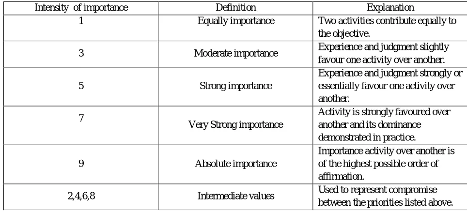
Step-5 The acceptable Degree of preference Definition Explanation: TABLE-1: SAATY 1-9 SCALE:
Intensity of importance Definition Explanation
1 Equally importance Two activities contribute equally to
the objective.
3 Moderate importance Experience and judgment slightly
favour one activity over another.
5 Strong importance
Experience and judgment strongly or essentially favour one activity over another.
7
Very Strong importance
Activity is strongly favoured over another and its dominance demonstrated in practice.
9 Absolute importance
Importance activity over another is of the highest possible order of affirmation.
2,4,6,8 Intermediate values Used to represent compromise
[image:3.612.63.545.274.495.2]between the priorities listed above.
Table 2 : Random Consistency Index ( RI)
CR range varies according to the size of matrix i.e. 0.05 for a 3 × 3 matrix, 0.08 for a 4 ×4 matrix and 0.1 for all larger matrices, n > 5. If the value of CR is equal to, or less than that value, it implies that the evaluation within the matrix is acceptable or indicates a good level of consistency in the comparative judgments represented in that matrix. In contrast, if CR is more than the acceptable value, inconsistency of judgments within that matrix has occurred and the evaluation process should therefore be reviewed, reconsidered and improved.
B. The Methodology Involves The Following Steps:
1) Development of a hierarchical structure of maintenance selection criteria.
2) Performing AHP analysis through pair-wise comparisons.
3) Defining objective function and constraints of the problem at hand using goal programming based on global and local AHP scores.
4) Selection of appropriate maintenance policy.
n 1 2 3 4 5 6 7 8 9 10
C. Development of Hierarchical Structure of Maintenance Selection Criteria
The first step in the development of AHP–GP model is the identification of maintenance criteria that would be taken into consideration for maintenance policy selection. Structuring the problem into hierarchy serves two purposes. First, it provides an overall view of the complex relationship of variables inherent in the problem and second. It helps the decision maker in making judgment on comparison of elements that are homogeneous and are on the same level of the decision hierarchy. A four level hierarchical structure is developed for the proposed model. The top level represents the goal of the analysis (selection of maintenance policy), the second level considers the criteria namely consequence of failure, and cost of maintenance policy, and the second level defines the sub criteria and fourth level possible alternative maintenance policies. The hierarchy scheme for the maintenance policy selection is shown in FIGURE-2.
FIGURE-3: The hierarchy scheme for the maintenance policy selection
D. Performing AHP Analysis
The AHP analysis comprises:
1) Collection Of Data For Pair-Wise Comparison: In order to collect pair-wise comparison data for criteria considered and for alternative maintenance policies based on criteria, four experts in the field (two from maintenance and two from operations having coordination with maintenance) were asked pertinent questions. For pair-wise comparison between the two criteria, the question asked was:
a) Question A: To select an appropriate maintenance policy for the process equipment present in the sms , we have identified two main criteria elements:
i) Consequence of failure and
ii) Cost of the maintenance policy.
Which of these two criteria elements of greater importance (priority) to you in the appropriate maintenance policy selection and how much? Based on his knowledge and experience the expert gives an answer with a quantitative value (or values) to help create a pair-wise comparison matrix amongst the given criteria. Once a comparison scale was provided to the experts for providing their responses. A 9-point scale was constructed as provided by Satty (1980), the scale is given above in Table-5. Every input is rated on a 1–9 judgment scale to determine relative importance of the different attributes on one level of the hierarchy to one another. To compare ith criteria with jth criteria, the decision maker assigns a value aij, which corresponds to a numerical value, an integer in range 1–9 as shown in Table-5.
2) Estimating Global and Local Scores: The crux of AHP is the determination of the relative weights to rank the decision alternatives. The steps to be followed for performing AHP analysis are given below.
a) Compare and rank the criteria failure and cost based on the order of importance.
b) Normalized the ranks to obtain relative weights for risk and cost.
c) Select the first criterion, risk for ranking the maintenance policies.
d) Select the first pair of maintenance policies, corrective maintenance (CM) and time-based maintenance (TBM) for comparison.
e) Rank CM with respect to TBM from the risk point of view.
f) The rank of TBM with respect to CM is the reciprocal of the
g) rank given in step (iii) above.
i) Value of rating judgements.
j) Verbal judgements.
i) aij = 1 The two parameters are equally important 3 Parameter i is weakly more important than parameter j,
ii) aij = 5 Parameter i is strongly more important than parameter j,
iii) aij = 7 Parameter i is very strongly more important than parameter j,
iv) aij = 9 Parameter i is absolutely more important than parameter j.
v) 2, 4, 6, 8 Interval values between two adjacent choices
k) Next, select TBM and rank it with respect to all maintenance alternatives from CBM onwards.
l) Tabulate the data. The diagonal values will be equal to one.
m) Normalize the ranks across the columns so that each column sums to one by dividing each element of a column by the corresponding column sum.
n) Calculate the average for each row. The average obtained is the relative weight for each maintenance alternative for risk. The relative weights are the local scores.
o) Repeat the steps (iii) to (ix) for the cost.
p) Compute global score for each maintenance policy by summing the products of weight of maintenance selection criteria (e.g., failure) and corresponding local score of the maintenance policy.
On completion of the above mentioned steps, the following outputs will be obtained:
i) Weights of maintenance policy selection criteria.
ii) Global scores for maintenance policy.
iii) Local scores at each level.
3) Evaluation Of Consistency Of The Comparison Matrix: Although perfect consistency is hard to achieve especially when considering multiple conflicting criteria, AHP provides a mechanism of measuring the consistency of the decision made, and allows for revisions of the decision in order to reach an acceptable level of consistency. AHP measures the consistency of judgment by means of Consistency Ratio (CR). A value of 10% or less is accepted as a good consistency measure. If the value exceeds 10 percent, it means that the judgment may somehow be random and should be revised (Saaty, 1980). Calculating the CR starts with multiplying each entry of the pair-wise comparison matrix by the relative priority (the average) corresponding to the column, and then totalling the row entries. Next, the row totals are divided by the corresponding entry from the priority vector. The average of those entries is the Eigen value kmax.
a) Consistency Index (Ci) For An N Elements Matrix Is: The CI is then divided by its random index (RI) to get the consistency ratio, which is a measure of how much variation is allowed. Computer software based on the AHP principles, Expert Choice, is available for evaluation and analyses.
4) Development Of Goal Programming Model: The global and local priority of the different possible maintenance policies with respect to each second level criterion namely risk contribution and cost are obtained through AHP analysis. These outcomes of AHP are embedded in Goal Programming (GP) to develop the AHP–GP model. The final result is a vector, normalized to the unity that allows identifying the better alternative with respect to the target (Bertolini and Bevilacqua, 2006). The priority of alternate policies and criteria namely risk and cost are adopted for the development of optimal maintenance policy selection model. In this goal programming model, three goals, namely global scores of maintenance policies, local scores of maintenance policies based on consequence of failures, and local scores of maintenance policies based on cost are set. All the three goals are stated below.
a) Goal1: Maximize global scores of maintenance policies.
b) Goal2: Maximize local scores of maintenance policies based on Consequence of failure.
c) Goal3: Maximize local scores of maintenance policies based on cost. Where,
d_k, dþk – Deviations from the target for kth criteria,
xi – Alternative ith maintenance policy such as corrective maintenance, time-based maintenance, condition based maintenance,
IV. MODEL CALCULATIONS
In this chapter an effort is made to apply the data collected from SMS department of Visakhapatnam steel plant for the methodology described in the previous chapter consists of
A. Calculation Of Dependence Among The Data Criteria
Table-3: Periodicity
1 2 3 4 5 6
PERIODICITY CM TBM CBM RCM WEIGHTS (WI) WI*TI
CM 1 0.143 0.167 0.143 0.047 0.990
TBM 7 1 2 4 0.492 0.931
CBM 6 0.5 1 2 0.276 1.011
RCM 7 0.25 0.5 1 0.185 1.325
TOTAL (TI) 21 1.893 3.667 7.143 1 4.256
1) Description of table-3: In the above table-3: The first column of first element is 1 and it represents when two activities contribute equally to the objective so its value is one. Hence the equal importance given to CM to CM.
2) According To Saaty 9 Points (Table-1 Page No :)
a) In the first column of second element is 7 represents and it when experience and judgment slightly favor one over the another. So its value is 7. Hence the moderate importance given to the TBM to CM.
b) In the first column of third element is 6 represents and it when experience and judgment slightly favor one over the another. So its value is 6. Hence the moderate importance given to the CBM to CM.
c) In the first column of fourth element is 7 represents and it when experience and judgment slightly favor one over the another. So its value is 7. Hence the moderate importance given to the RCM to CM.
d) In the second column of first element is 1/7=0.143 and it represents reversing comparison of CM to TBM so its value is 1/7. A reciprocal value automatically assigned to the reverse comparison.
e) In the third column of first element is 1/6=0.167 and it represents reversing comparison of CM to TBM so its value is 1/6. A reciprocal value automatically assigned to the reverse comparison.
f) In the fourth column of first element is 1/7=0.143 and it represents reversing comparison of CM to TBM so its value is 1/7. A reciprocal value automatically assigned to the reverse comparison.
g) In the third column of second element is 2 represents and it when experience and judgment slightly favor one over the another. So its value is 2. Hence the moderate importance given to the TBM to CBM.
h) In the second column of third element is 1/2=0.5 and it represents reversing comparison of CM to TBM so its value is 1/2. A reciprocal value automatically assigned to the reverse comparison.
i) The fourth column of fourth element is 1 and it represents when two activities contribute equally to the objective so its value is one. Hence the equal importance given to RCM to RCM.
j)In this manner all the remaining elements in 1st, 2nd, 3rd and 4th columns are calculated.
3)Calculations Of Weights Of Criteria: The first element of 5th column is 0.047 is obtained in the following manner it average of following 4 values each of which is calculated in following manner:
a)The first value = first element of first row/total of all the elements in first column = (1)/(1+7+6+7) = 1/21 = 0.0476
b) The second value = second element of first row/total of all the elements in first column = (0.143)/(0.143+1+0.5+0.25) = 0.0755
c) The third value = third element of first row/total of all the elements in first column = (0.167)/(0.167+2+1+0.5) = 0.0455
d) The fourth value = fourth element of first row/total of all the elements in first column = (0.143)/(0.143+4+2+1) = 0.02.
e) The average of all the four values
= (0.0476+0.0755 +0.0455+0.02)/4 = 0.047 (5th column first element).
4)Calculation of Wi*Ti
a)The value in column six are obtained in the following manner
b) The 1st element in the 6th column (0.990) = 0.047 (The 1st element in the 5th column) * 21 (total of all the elements in first column).
= 0.990 (6th column first element).
c)The 2nd element in the 6th column (0.931) = 0.492 (The 2nd element in the 5th column) * 1.893 (total of all the elements in 2nd column).
= 0.931 (6th column 2nd element).
d)The 3rd element in the 6th column (1.011) = 0.276 (The 3rd element in the 5th column) * 3.667 (total of all the elements in 3rd column).
= 1.011 (6th column 3rd element).
e)The 4th element in the 6th column (1.325) = 0.185 (The 4th element in the 5th column) * 7.143 (total of all the elements in 3rd column). = 1.325 (6th column 4th element).
5)Calculation Of Consistency Ratio
Nmax = 4.256 (6th column last element). n = 4 (order of matrix).
Consistency Index (CI) = (Nmax-n)/(n-1) = (4.256-4)/(4-1) = 0.08534 Random Consistency Index (RI) = 0.9 (from saaty table-2 page)
Consistency Ratio (CR) = CI/RI
= 0.08534/0.9 = 0.09482 From the above table: 0.05x1+ 0.49x2+0.27x3+0.19x4 ---- 1
Note: In this manner all the constraint equations calculated.
TABLE-4:DOWN TIME
1 2 3 4 5 6
DOWN TIME CM TBM CBM RCM Wi wi*ti
CM 1 0.142857 0.333333 0.166667 0.06262 1.064544
TBM 7 1 0.5 0.5 0.241853 1.243817
CBM 3 2 1 0.5 0.26425 1.012957
RCM 6 2 2 1 0.431277 0.934433
TOTAL(ti) 17 5.142857 3.833333 2.166667 1 4.255751
From above table: 0.06x1+ 0.24x2+0.26x3+0.44x4 ---- 2
TABLE-5: PRODUCTION
From above table: 0.05x1+ 0.14x2+0.56x3+0.25x4 ---- 3
1 2 3 4 5 6
PRODUCTION CM TBM CBM RCM Wi Wi*Ti
CM 1 0.25 0.142857 0.166667 0.0517 0.930601
TBM 4 1 0.2 0.5 0.142474 1.175409
CBM 7 5 1 3 0.558599 0.936319
RCM 6 2 0.333333 1 0.247227 1.153725
TABLE-6: QUALITY
1 2 3 4 5 6
QUALITY CM TBM CBM RCM Wi Wi*Ti
CM 1 0.2 0.25 0.142857 0.055665 0.946307
TBM 5 1 0.5 0.333333 0.18622 1.154567
CBM 4 2 1 0.333333 0.238153 1.131226
RCM 7 3 3 1 0.519962 0.940883
TOTAL(Ti) 17 6.2 4.75 1.809524 1 4.172983
From above table: 0.06x1+ 0.18x2+0.24x3+0.52x4 ---- 4
TABLE-7: SAFETY
1 2 3 4 5 6
SAFETY CM TBM CBM RCM Wi Wi*Ti
CM 1 0.166667 0.2 0.142857 0.049721 0.944691
TBM 6 1 2 0.333333 0.250239 1.167782
CBM 5 0.5 1 0.25 0.163504 1.177231
RCM 7 3 4 1 0.536536 0.926163
TOTAL(Ti) 19 4.666667 7.2 1.72619 1 4.215868
From above table: 0.05x1+ 0.25x2+0.16x3+0.54x4 ---- 5
TABLE-8: SERVICE LEVEL
1 2 3 4 5 6
SERVICE LEVEL CM TBM CBM RCM Wi Wi*Ti
CM 1 0.142857 0.25 0.2 0.053475 0.909077
TBM 7 1 5 4 0.586846 0.934761
CBM 4 0.2 1 0.5 0.142447 1.175184
RCM 5 0.25 2 1 0.217233 1.238227
TOTAL(Ti) 17 1.592857 8.25 5.7 1 4.257248
From above table: 0.05x1+ 0.59x2+0.14x3+0.22x4 ---- 6
TABLE-9: POLICY
1 2 3
POLICY EFFECT COST Wi
EFFECT 1 5 0.83
COST 0.2 1 0.17
TOTAL(Ti) 1.2 6 1
TABLE-10: COST
1 2 3
COST DOWNTIME PERIODICITY Wi
DOWNTIME 1 4 0.8
PERIODICITY 0.25 1 0.2
TABLE-11: EFFECT
1 2 3 4 5 6
EFFECT PRODUCT QUALITY SAFETY SERICELEVEL Wi Wi*Ti
PRODUCT 1 0.5 0.2 5 0.164304 1.347296
QUALITY 2 1 0.333333 3 0.209291 1.011572
SAFETY 5 3 1 7 0.566134 0.948949
SERVICELEVEL 0.2 0.333333 0.142857 1 0.060271 0.964332
TOTAL 8.2 4.833333 1.67619 16 1 4.272149
Global Scores at Effect Level
Where
The 5th column elements are from table-11 (Wi) column elements.
The second column elements are from table-5 (Wi) column elements.
The 3rd column elements are from table-6 (Wi) column elements.
The 4th column elements are from table-7 (Wi) column elements.
The 5th column elements are from table-8 (Wi) column elements.
The 6th column elements are getting by multiplying relative importance of criteria by associated weights.
TABLE-12: global scores at effect level
Wi 0.05152 0.23942 0.24277 0.46629
G
1 2 3 4 5
1 0.8 0.2 wi
2 0.047136 0.06262 0.037709 0.012524 0.050233
3 0.491772 0.241853 0.393418 0.048371 0.441789
4 0.275648 0.26425 0.220519 0.05285 0.273368
5 0.185443 0.431277 0.148354 0.086255 0.23461
TOTAL 1 1 0.8 0.2 1
Where
The 3nd column elements are from table-9 (Wi) column elements.
The 1st column elements are from table-12 (wi) column elements. The 2nd column elements are from table-13 (wi) column elements.
The 4th column elements are getting by multiplying relative importance of criteria by associated weights. From above table: 0.05x1+ 0.27x2+0.25x3+0.46x4 ---- 7
B.Solving The Goal Programming
1)Minimize: y7- + y6- +y5- + y4- + y3- + y2- + y1- .
Subjected to
0.05x1+ 0.49x2+0.27x3+0.19x4- y1++ y1- = 0.76 --- > 1
0.06x1+ 0.24x2+0.26x3+0.44x4- y2++ y2- = 0.70 --- > 2
0.05x1+ 0.14x2+0.56x3+0.25x4- y3++ y3- = 0.81 --- > 3
0.06x1+ 0.18x2+0.24x3+0.52x4- y4++ y4- = 0.70 --- > 4
0.05x1+ 0.25x2+0.16x3+0.54x4- y5++ y5- = 0.79 --- > 5
0.05x1+ 0.59x2+0.14x3+0.22x4- y6++ y6- = 0.81 --- > 6
0.05x1+ 0.27x2+0.25x3+0.43x4- y7++ y7- = 1.00 --- > 7.
Where x1 is Corrective maintenance (CM),
x2 is Time based maintenance (TBM),
x3 is Condition based maintenance(CBM),
x4 is Reliability centered maintenance(RCM).
Solution
X1 (CM) 10.9766
X2 (TBM) 00.6713
X3 (CBM) 00.0000
X4 (RCM) 01.0070
2) Result: The highest value of the above solutions are x2, x2 is TBM (Time based maintenance) is =10.3883.
a) From above result gives Time based maintenance is the most effective maintenance for trunion ring.
V. RESULTS
The case study is done for the components of LG converter detail methodology and calculation is illustrated for one component. Similarly for all components, same calculations are done for other components.
The AHP–GP model provides some interesting results. The AHP provides local and global scores based on which meaningful inferences can be drawn. While local score weighs the policies based on criteria, the global score combines the local scores. GP model (goal programming model) takes into consideration all the three scores and decides the most appropriate maintenance policy for each considered equipment. The findings are tabled below
COMPONENT EXISTING PROPOSED
TRUNION RING CM CM
REDUCER TBM CBM
FLOATING BEARING TBM TBM
LUBRICATION SYSTEM TBM RCM
VI. CONCLUSIONS
AHP- GP model has considered all the criteria and simultaneously priotioritising local and global scores. The results are discussed among site personnel and found satisfactory.
While comparing present with proposed these factors were viewed:
1) Cost of mentoring equipment and benefit if CBM is adopted.
2) If corrective maintenance is adopted production gain with respect to time of shutdown required for maintenance.
3) If RCM is adopted reduction in MTBF.
4) If TBM is applied production effect, cost of spares required additionally. *The prosed method is addressing all these issues. Hence it is suggested to adopt*.
VII. ACKNOWLEDGEMENTS
I would like to express my deep sense of my gratitude and indebtedness to Dr. V.V.S KESAVA RAO, A. U. College of Engineering for his inspiring guidance, valuable suggestions and constant encouragement throughout my thesis work. I owe him lots of gratitude for having me shown this way of work.
I am thankful to Prof. B. S. K. SUNDARASIVA RAO, Head of the Department, Department of Mechanical Engineering, for providing all the necessary facilities and encouragement for the present work. I also thank all the Mechanical engineering faculty members for sharing with my views and for their constant help extended in making my thesis work.
I wish to express deep sense of gratitude to M. SRINIVAS RAO, department of MMSM, Visakhapatnam Steel Plant, and Visakhapatnam. His invaluable and lucid suggestions and also his keep interest in my work served as an impetus for me. J. SUBASH KUMAR.
REFERENCES
[1] Saaty TL. The analytic hierarchy process. New York,NY:McGraw-Hill; 1980.
[2] Saaty TL. An exposition of the AHP in reply to the paper ‘Remarks on the Analytic Hierarchy Process’. Manag Sci 1990;36(3):259–68. [3] Lin WT. A survey of goal programming applications. Omega 1980; 8:115–7.
[4] Badri MA. A combined AHP-GP model for quality control system. Int J Prod Econ 2001;72:27–40.
[5] Kelly A. Maintenance organizations & systems: business-centered maintenance. Oxford: Butterworth-Heinemann; 1997. [6] Moubray J. Reliability centred maintenance. Oxford: Butter Worth- Heinmann Ltd; 1991.
[7] Smith AM. Reliability centred maintenance. New York, NY: McGraw-Hill; 1993.