An RSSI-based Wireless Sensor Network Localization
Algorithm with Error Checking and Correction
https://doi.org/10.3991/ijoe.v13i12.7892
Bo Guan, Xin Li!!"
School of Foreign Language, Beihua University, Jilin, China
Abstract—This paper studies the wireless sensor network localization algo-rithm based on the received signal strength indicator (RSSI) in detail. Consider-ing the large errors in rangConsider-ing and localization of nodes made by the algorithm, this paper corrects and compensates the errors of the algorithm to improve the coordinate accuracy of the node. The improved node localization algorithm per-forms error checking and correction on the anchor node and the node to be measured, respectively so as to make the received signal strength value of the node to be measured closer to the real value. It corrects the weighting factor by using the measured distance between communication nodes to make the coordi-nate of the node to be measured more accurate. Then, it calculates the mean de-viation of localization based on the anchor node close to the node to be meas-ured and compensates the coordinate error. Through the simulation experiment, it is found that the new localization algorithm with error checking and correc-tion proposed in this paper improves the localizacorrec-tion accuracy by 5%-6% com-pared with the weighted centroid algorithm based on RSSI.
Keywords—wireless sensor network, RSSI-based localization algorithm, rang-ing correction, error checkrang-ing and correction
1
Introduction
In recent years, many domestic and foreign research enthusiasts have carried out in-depth studieson the WSN localization algorithm. Juan [1]. proposed a WSN dis-tributed localization method based on local spatial constraints, which estimates the coordinate of a sensor node by using a program to constantly iteratively solve a set of local spatial constraintsand then constantly updates it based on the adjacent nodes in the communication range. ThuL [2]. proposed a compressed sensing localization method based on deterministic sensing matrix, which defines multiple sensor nodes as a sparse matrix in a discrete region, recovers noise measurement withthe received signal strength information, and then locates the target. Jian [3]. proposed a cluster-based WSNlocalization algorithm, which uses the cluster structure and a global sys-tem to represent the logic of the network andreduces measurement errorsbased on the probability of multi-hop, so as to improve the localization accuracy of nodes. Qiao Xin et al. [4]. proposed using percentage to correct the average hop distance of anchor nodes in DV-Hop, and used the differential particle swarm optimization algorithm to optimize the location coordinates of the nodes to be measured. WenJiangtao et al. [5]. analyzed the defects and shortcomings of the classical DV-HOP algorithm, used a quantization model to represent node errors and finally utilized the weighting factor to correct the location coordinates of the nodes. Cui Fayi [6]. proposed the quadrilateral localization algorithm, which selects the four anchor nodes with the least path loss, performs combination ranging of three of them and takes the average of the coordi-nates obtained from the qualified triangles as the location coordinate of the node to be measured, which improves the accuracy to a certain extent.
By comparing different localization algorithms, this paper finds that the RSSI-based localization algorithm has a high accuracy and there is no need for additional hardware, so this paper further studies the RSSI-based WSN localization algorithm, aiming to reduce the measurement errors in the ranging and localization of sensor nodes and improve the localization accuracy of the nodes to be measured.
2
Analysis of the anchor node localization algorithm
2.1 Establishment of the network model
At present, popular network models include the free space propagation model, hata model, log-distance distribution model and log-distance path loss model. This algo-rithm integrates all the above models. The free space propagation model is as follows:
!" ! ! !"!!!!! !"# !"! ! !!!! !! (2)
where, PL(d) represents the path loss after distance d, !!represents the Gaussian-distributed random variable with a mean of 0, and its standard deviation is between 4-10; k ranges from 2 to 4. Suppose d=1m, then substitute it into Formula (2) to obtain the valueof!"!!!!. So when each anchor node receives the signal, the signal strength
is calculated as below:
!""# ! ! ! ! !!"!!! (3) In the above equation, P represents the transmission power; and G represents the antenna gain. The error in the absolute distance produced by the deviation of the RSSI value decreases as the distance from the node to the signal source shortens. This is because, due to the impact of !!, the RSSI fluctuation causes the absolute distance
error to become larger, which in turn results in an increase in the RSSI value.
2.2 Distance estimation based on RSSI
Assuming that in the ideal case, the received signal strength indicator between the two nodes decreases with the increase of the distance - the longer the distance, the smaller the strength, so the distance between two nodes corresponding to the mini-mum received signal strength is the longest. When all the RSSI values in the entire network are collected, find the minimum value in the set C of the RSSI values, as shown in the following formula:
!!"#!!!"#! !"#!!!!!!!!!!!!!! (4)
Then the distance between the nodes corresponding to!!"# is the longest, denoted
as!!"#, and the distance !!!! !! between the two nodes corresponding to the edge
!!!! !! is denoted as:
!!"! !!"#
!!"!!!
!!"#!!! (5)
Since !!"# represents the maximum value of the distance between communicable nodes in the entire network, if the distance between the two nodes is large enough, they will not be able to communicate again as they cannot receive signals from each other and!!"#will becloser to the communication radius R of the wireless sensor network node.So the value of !!"# is approximately equal to R in the algorithm and the estimated distance of the edge !!!! !! is obtained as follows:
!!"#$%! !
!!"!!!
!!"#!!! (6)
!!".Such an approximate estimate will result in some error in the localization algo-rithm.
In addition, the localization algorithm also eliminates !! when it finds the relative relationship between each localization node. !! represents the scale factor between the path length and the path loss in the wireless signal propagation model. The values of !! are different depending on the environment. If the scale factor is eliminated, the observer will be able to estimate the distance between the nodes with the value of
!!unknown, which will bring many benefits to the algorithm. Therefore, this distance
estimation algorithm can be applied in any environment, and, with this algorithm, we can also deduce the value of !!, as shown below:
!!!!" !"#!!!!!"!"!!"!!"!!!"#!!!"#!"! (7)
where R represents the communication radius of the sensor localization node. This result can also be used as an angle to observe the unknown environment when the sensor node is deployed in an unknown area.
2.3 Error correction analysis of anchor nodes
The error of the beacon node is obtained through comparison of the distance value measured by RSSI and the actual measured one. Take an anchor nodewith known coordinates as the node to be measured, calculate its coordinates by the trilateration method and then compare them with the actual coordinates to obtain the errors. So during the localization of an anchor node, if both errors are taken into account, the impacts of the interference factors in the network can be reduced. Suppose the adap-tive weighted correction coefficient for the RSSI ranging of anchor node is as follows:
! ! !!!!!!!!!!! (8)
where, !! !!! !
!" !!!!!!!"!
!
!!! !!!!!!!is the adaptive weighted factor, representing the weight of each RSSI measured value. !!! !!!! !!!!!!!", where !!stands for the
measured distance between the anchor nodes to be corrected and i stands for the num-ber of anchor nodes used for correction. For each anchor node in the entire network, the location information of other anchor nodes can always be used to correct its RSSI measured value.µ can reflect theRSSI measurementaccuracy ofthe anchor nodes.
The correction distance between the anchor nodesto be measured can be expressed as:
and partition in the trilateration, so anchor node information needs to be used for further correction. The coordinate errors of the anchor node can be expressed as:
!!"! !!! !!"
!!"! !!! !!" (10) where !! represents the actual X-coordinate value of the j-th anchor node; !!" repre-sents the calculated X-coordinate value of the j-th anchor node; !!represents the actual Y-coordinate value of the j-th anchor node; !!" represents the calculated Y-coordinate
value of the j-th anchor node. The calculated coordinate errorsof the anchor node are the localization errors of the network where the anchor node is located. The network localization errors can be expressed as:
!!!!! !!!!!!"
!!!!! !!!!!!"
(11)
where !! ! ! !!!!!"denotes the X coordinate error of the j-th node; and!!" denotes the Y coordinate error of the j-th node. The network localization error is actually the mean value of the anchor node coordinate localization errors, so the final coordinates of the anchor node to be measured can be expressed as:
! ! !!! !!
! ! !!! !! (12)
where !! is the X-coordinate of the anchor node to be measured by the trilateration method; !! represents the calculated Y-coordinate of the anchor node to be measured.
The above analysis shows that the distance between each anchor node is measured by the known anchor nodes. µ represents the measurement error coefficient of the anchor nodes, and it is used only to correct the distances calculated by anchor node measurement.
3
Error analysis of the node to be
measured
3.1 Errors in distance estimation
Errors in measurement of the RSSI value. The ideal RSSI value between two sensor nodes i, j, which can communicate with each other, is denoted as!!", and the measured RSSI value isdenoted as!!".Here the Gaussian random variable is used to fit the signal interference in the real environment to obtainan analog value.!!"can be expressed in the formula below:
!!"! !!"!!! (13)
where !! is the Gaussian random variable with a mean of0 and a variance of !, and
!! will vary within the corresponding range. Therefore, when the distance between i
and j increases, the energy value !!" it receives will be smaller. As can be seen from Formula (13), when !!" is small, the error of the corresponding!!"will be greater, so in actual practice, we may calculate the mean of RSSI values between two communica-ble nodes to reduce the error caused by the RSSI ranging.
Assuming that the true distance between i and j is !!" and that the estimated dis-tance through calculation is denoted as!!", then according to Formula (5), the distance between two communication points can be obtained, as shown in Formula (14):
!!"=!!"#
!!"!!!
!!"#!!! (14)
Here we can approximately take!!"#! !, where R represents the communication radius of the sensor localization node, but in reality,!!"#! !, so this approximate value will also bring some error to the estimated distance. If after one of the RSSI value measurement, !!" and !!"# are known, then R can be approximated to be the
error of the maximum distance between communicable nodes. Assuming that
!!"#! !!!! ! ! ! !!, Formula (14) can be obtained as follows:
!!"! !!!"#!!!!!"!!! !!!"#!!!!!"!!! ! !!!!"!!!!"#!!!! !!!"#!!!!!"!!! ! ! !!!"#!!!!!"!!!
! !!!"#!!!!!"!!! ! !! (15)
Then,!!!!!!!!!"!!!!"#!!!! !!! !!"!!!
!!"#!!! (16)
Formula (16) is the error produced by R beingapproximated as!!"#, and from the
formula, it can be seen that !! itself involves the measurement error of RSSI value, so
errors will be accumulated in the calculation process of !!".
Errors produced by the approximation of the communication radius R of WSN nodes and the maximum distance between communicable nodes. The rela-tionship model between RSSI and distance can be expressed as a quadratic polynomi-al, i.e.!""#! !!!"#$%&! !, where a is the coefficient to be determined and length is the
distance. In this Gaussian model, there must be sensitive and non-sensitive regions, and the sensitive region refers to the RSSI value rangewithin which any value will cause a great change in the distance. When the measured RSSI value is within this sensitive region, the error produced by the calculated distance will be larger; other-wise, the error will be reduced.
3.2 Errors in location calculation
algorithm, and instead, it adopts the cross method. Using different planning solutions will result in different localization errors.
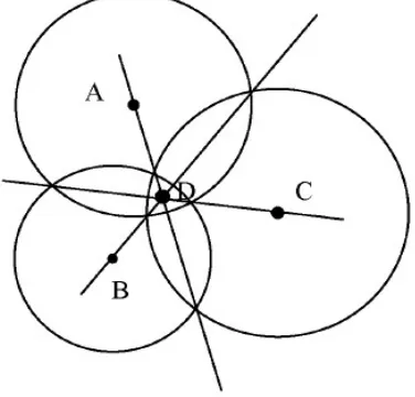
Signals will be attenuated in the process of propagation, so ranging through the RSSI value will produce errors in distance, and asa result, the three circles do not always intersect at one point in the trilateration method.The actual situation may be similar to the result shown in Figure 1.
Fig. 1. Trilateration in actual situation
It can be seen from Figure 1 that, the actual measurement is somewhat different from the ideal result, which isaffectedby environmental factors.
The impacts of the external environment on the RSSI value are also relatively large, as there are alwaysunstable factors.Different application environments have different error interferences, and the application environment for localization nodescontain many variable factors, which affect the wireless signal transmission of the nodes.
In summary, it can be seen that both the location calculation error and the localiza-tion calculalocaliza-tion error can be reflected in error checking and correclocaliza-tion by the planning problem solution method.
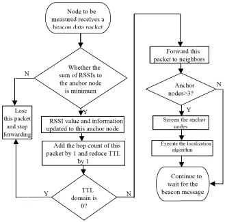
3.3 Design of the localization algorithm for nodes to be measured with error checking and correction
Fig. 2. Flowchart of the localization algorithm for nodes to be measured
3.4 RSSI ranging correction model analysis
The RSSI technology is a localization technology used to calculate the location of a node by the propagation model of radio frequency signals. It mainly estimates the distance between the node to be measured and multiple anchor nodes by the degree of signal attenuation, and then estimates the coordinates of the node to be measured based on the calculated distance. In practical practice, the diffraction of radio waves are affected by multiple paths, thereby reducing the localization accuracy. We set the coordinates of all anchor nodes as !!!! !!!, and the coordinates of the node to be measured as!!!! !!, which along with the surrounding anchor nodes can determine different circles, as shown in the following formula:
!!! !!!! !!!! !!!! !!!(i=1,2,…M) (17)
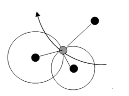
If the interference of noise is not considered, the intersection of these circles will be the coordinates of the node to be measured, as shown in Figure 3.
The locations of the anchor nodes are fixed, so the distance between any two an-chor nodes is constant, andrelative to the plane system, the node to be measured will be localized on the hyperbola with the two anchor nodes as the intersections, as shown in Formula (18):
!!!!! !!! !!! !!! ! !! !!!! !! !!!! !!!! !!!! !!! (18)
Fig. 3. Intersections of circles
RSSI valuesreceived by the node, and find three anchor nodes with the strongest RSSI values among the surrounding ones, and then it calculates the coordinates of the node to be measured using trilateration and other related algorithms. Secondly, the anchor node with the highest RSSI value is shielded, and the remaining two anchor nodes and the next anchor node with ahigh RSSI value form a triangular region. In this way, the new coordinates of the node will be calculated through the localization algorithm and the offset direction of the node can be determined. Then again, the anchor node with the highest RSSI value is removed from the anchor nodes. Each time the node shifts for a certain distance, the localization will be repeated to achieve a higher localization accuracy.
4
Comparison and analysis of experimental results
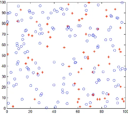
4.1 Deployment of communication nodes
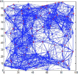
In order to test the performance of the proposed localization algorithm, the im-proved localization algorithm and several other localization algorithms are simulated and verified on the Matlab software test platform. First, all the anchor nodes and the nodes to be measured are randomly distributed in the 100m"100m square monitoring region, with the communication radius of the radio frequency being R and the exper-imental path loss coefficient n being set to 3. Due to the impacts of obstacles and reflection in the actual environment, themean square deviation of Gaussian distribu-tion is introduced and set as 2. As shown in Fig.4, 200 sensor nodes are randomly and evenly distributed in the square simulation area,including 60 anchor nodes and 140 nodes to be measured. The blue o indicates the nodes to be measured, and the red * indicates the anchor nodes.
The improved localization algorithm and the comparative localization algorithms are applied to the monitoring region respectively to understand the characteristics of each algorithm and the improved performance.
4.2 Simulation of the improved algorithm
Through the design and deployment of the monitoring region, sensor nodes are randomly distributed in the square monitoring region. Each node has its own commu-nication range and scans other nodes in the commucommu-nication range to communicate. Data are exchanged between nodes through communication. The sensor node can obtain the location relations with other nodes within its communication radius, and then uses the appropriate ranging method to calculate the neighbor relation graph to determine whether the anchor nodes around it satisfy the localization requirements. Then the node localization is carried out, as shown in Figure 5.
Fig. 5. Neighborhood chart of randomly distributed nodes
In the localization process, the most important evaluation criterion for an algorithm is the average localization error, so it is necessary to normalize the average localiza-tion error. The average error formula is as follows:
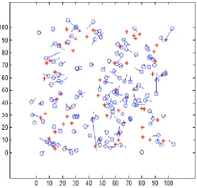
Where N is the number of nodes to be measured, R is the communication us,!!!!! !!! is the actual value of the node to be measured and!!!!! !!!! is the measured value of the node to be measured. Therefore, thelocalization error of each node can be obtained from the estimated localization and the actual location of the node to be measured, as shown in Figure 6.
Fig. 6. Localization errors under random node distribution
Figure 6 shows the localization error diagram of the improved localization algo-rithm in the square simulation region. Through calculation of the neighbor relation-ships between nodes, the location coordinates of the nodes to be measured are located and the corresponding errors are generated. The red * denotes the anchor nodes, the blue o denotes the nodes to be measured and the blue lines are the localization errors of the nodes.
4.3 Experimental results analysis
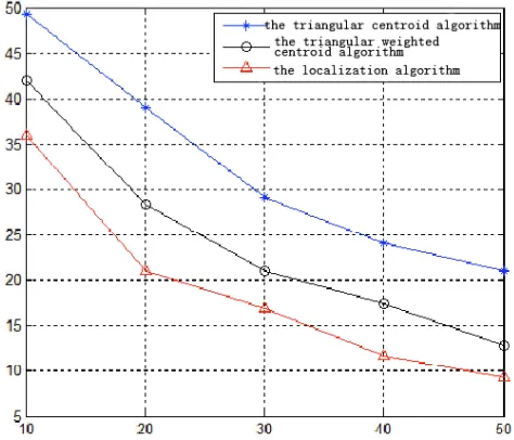
anchor node numbers. When the total number of nodes is 100 and the communication radius is 20cm, the number of anchor nodes is increased gradually from 10 to 50. From this figure, it can be seen that, when the number of anchor nodes increases, the average localization errors of the nodes to be measured decrease. When there are 10 anchor nodes, the average localization error of the original localization algorithm is around 49% while that of the improved algorithm proposed in this paper is around 37%. When there are 50 anchor nodes, the average localization error of the original algorithm is around 22% and that of the improved one is about 9%. In summary, the improved algorithm proposed in this paper reduces the average localization error by about 12% and the average localization error is 5% less than those of other improved algorithms.
Fig. 7. Number of anchor nodes and average error
5
Conclusions
Acknowledgment
This paper is the relevant research result of the Teaching and research project of Beihua University (No. XJQN2017011) and the Educational Science Program in Jilin Province "Research on the teaching model reform of Library Literature Retrieval Course under the prosperity of network culture"(No. GH170053).
References
[1]Cota-Ruiz (2013). A Distributed Localization Algorithm for Wireless Sensor
Net-works based on The Solutions of Spatially-Constrained Local Problems. IEEE Sensors Journal, 13(6), pp. 2181-2192. https://doi.org/10.1109/JSEN.2013.2249660
[2]Nguyen, T. L. N., Shin, Y. (2015). Multiple Target Larget Localization in WSNs based on Compressive Sensing Using Deterministic Sensing Matrices. International Journal of Dis-tributed Sensor Networks, 16, pp.1-8. https://doi.org/10.1155/2015/123982
[3]Shu, J. (2009). Cluster-based Three-dimensional Localization Algorithm for Large Scale Wireless Sensor Networks. Journal of Computers, 4(7), pp.585-592.
https://doi.org/10.4304/jcp.4.7.585-592
[4]Xin, Q. (2014). Modifying Average Hopping Distances Based Iterative Algorithm for Quasi-Newton in WSN. Chinese Journal of Sensors and Actuators. 27(6), pp. 797-801. [5]Wen, J. (2014). Improved DV-Hop Location Algorithm Based on Hop Correction, Chinese
Journal of Sensors and Actuators. 27(1), pp.113-117.
[6]Cui, F. (2015). Weighted Centroid Localization Algorithm based on Multilateral Localiza-tion Error of Received Signal Strength Indicator. Infrared and Laser Engineering. 44(7), pp. 2162-2168.
[7]Huang, X. (2014). Target Localization Based on Improved DV-Hop Algorithm in Wireless Sensor Networks, Journal of Networks,38(4), pp.393-422. https://doi.org/10.4304/jnw. 9.01.168-175
[8]Zhang, A. (2015). Wireless Localization based on RSSI Fingerprint Feature Vector. Inter-national Journal of Distributed Sensor Networks, 28(47), pp.1-7. https://doi.org/10.1155/ 2015/528747
[9]Pal, A. (2010). Localization Algorithms in Wireless Sensor Networks:Current Approaches and Future Challenges. Network Protocols and Algorithms, 2(1), pp. 45-73.
https://doi.org/10.5296/npa.v2i1.279
[10]Wu, G. (2012). A Novel range-free Localization Based on Regulated Neighborhood Dis-tance for Wireless ad hoc and Sensor Nteworks. Computer Networks, 56(16), pp. 3581-3593. https://doi.org/10.1016/j.comnet.2012.07.007
[11]Tan, G. (2013). Connectivity-based and Anchor-free Localization in Large-scale 2d/3d Sensor Netorks. ACM Transactions on Sensor Networks(TOSN), 10(1), pp.6-10.
https://doi.org/10.1145/2529976
[12]Mourad, F., Snoussi, H, Abdallah F, et al. (2009). Anchor-based Localization ViaInterval Analysis for Mobile ad-hoc Sensor Networks. Signal Processing, IEEE Transactions on, 57(8), pp.3226-3239. https://doi.org/10.1109/TSP.2009.2020018
[14]Zhang, X. (2015). An Efficient Algorithm for Localization Using RSSI based on ZigBee. Canadian Conference on Electrical and Computer Engineering, 3(6), pp. 366-369.
https://doi.org/10.1109/CCECE.2015.7129304
[15]Blumrosen, G. (2013). Enhanced Calibration Technique for RSSI-based Ranging in Body Area Networks.Ad Hoc Networks, 11(1), pp. 555-569. https://doi.org/10.1016/j.ad hoc.2012.08.002
[16]Yao, Y. (2015). A RSSI-Based Distributed Weighted Search Localization Algorithm for WSNs. International Journal of Distributed Sensor Networks, 29(3), pp.1-11.
https://doi.org/10.1155/2015/293403
6
Authors
Bo Guan is with the School of Foreign Language, Beihua University, Jilin, China.
Xin Li is with the School of Foreign Language, Beihua University, Jilin, China.