Comparative evaluation of daily evapotranspiration using
artificial neural network and variable infiltration capacity models
Sirisha Adamala
1*, Ankur Srivastava
2(1. Department of Applied Engineering, Vignan’s Foundation for Science, Technology and Research (VFSTR), Vadlamudi–522213, Guntur, Andhra Pradesh, India;
2. Agricultural and Food Engineering Department, IIT Kharagpur, Kharagpur-721302, India)
Abstract: Evapotranspiration is a key variable for hydrologic, climatic and agricultural studies. Accurate quantification of
this variable is the most important for irrigation management and crop productivity. With the availability of only meteorological data in climatic stations, reference gross evapotranspiration (ETo) estimation is becoming a challenging task. Hence, there is a scope to estimate the ETo using various physical and empirical methods. Among physical methods, FAO-56 Penman Monteith (PM) method is the best and Artificial Neural Network (ANN) model is an accurate empirical method. Further, ETo can also be estimated using a water budget approach i.e. variable infiltration capacity (VIC) model, which accounts for the sub-grid variability of land use, land cover and soil moisture accurately. In this study, the ETo was estimated by two different methods, namely, VIC and ANN for Mohanpur climatic location in India. The results of VIC-ETo showed the correlation coefficient, r = 0.853, coefficient of determination, R2 = 0.727 and index of agreement, d = 0.924; while ANN models with the FAO-56 PM method were in better agreement with r = 0.999, R2 = 0.998 and d = 0.999. Hence, it is concluded that the ANN showed better results as compared to VIC model for ETo estimation in Mohanpur climatic location.
Keywords: evapotranspiration, artificial neural network, model, climate, physical model
Citation: Adamala, S., and A. Srivastava. 2018. Comparative evaluation of daily evapotranspiration using artificial neural
network and variable infiltration capacity models. Agricultural Engineering International: CIGR Journal, 20(1): 32–39.
1 Introduction
Evapotranspiration is one of the significant components in the global hydrologic cycle. Accurate estimation of evapotranspiration is important for solving various crops, land, and water related problems.
Reference evapotranspiration (ETo) which mainly
depends on climate data is the basis for computing crop irrigation water requirements. There exists a direct measurement methods (lysimeters) and indirect estimation procedures (physical and empirical based) for modeling ETo. Many direct (lysimeters) and indirect
(empirical or semi-empirical) methods have been developed for estimating ETo as a function of climate
data.
Received date: 2017-04-27 Accepted date: 2018-01-20 * Corresponding author: S. Adamala, Assistant Professor,
VFSTR. Email: [email protected]. Ph: 2344700.
The globally accepted physically based FAO-56 Penman Monteith (PM) method indeed gives highly accurate estimates for ETo, but it requires detailed climate
data of air temperature, solar radiation, wind speed, and relative humidity (Debnath et al., 2015). Therefore, although are highly accurate, the FAO-56 PM model cannot be used for locations, where sufficient or reliable climatic data are not available, and in those cases the empirical or semi-empirical methods can be used, which require limited climate variables. However, empirical/semi-empirical methods are usually valid only for the local conditions under which they were derived, or when they applied to areas with climatic conditions similar to those for which they were developed (Kumar et al., 2002). Therefore, care should be taken not to use them outside the prescribed conditions.
specific climatic condition, and modelling nonlinear ETo
accurately based on weights sensitization (Adamala et al., 2014a, 2014b, 2015a, 2015b, 2016, 2017). But, at the same time, ANNs are producing the results without considering their physical meaning. Therefore, to estimate ETo, we need to consider physically based model,
i.e., Variable Infiltration Capacity (VIC). The VIC model (Billah et al., 2015, Liang et al., 1994, Srivastava et al., 2017) is a large-scale hydrology model that has been used to simulate land surface water and energy fluxes from the scale of large watersheds to global simulations. The advantages of this model over other hydrological model is that it incorporates the representation of sub-grid variability in soil infiltration capacity, vegetation classes and calculates the vertical energy with moisture flux in grid cell based on specification at each grid cell.
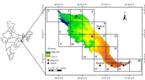
The Kangsabati River basin is selected herein as the study area to evaluate all the ETo estimation methods. The
Kangsabati River basin is located in the Indian state of West Bengal in between 86°00′E and 87°40′E longitudes and 22°20′N and 24°40′N latitudes having a geographical area of 5796 km2 (Figure 1). The elevation of this Kangsabati River basin ranges from 19 to 656 m above mean sea level. Paddy is the major crop grown in the cultivable land throughout the year in the three seasons of kharif, rabi and summer. The River basin receives an
average annual rainfall of about 1400 mm, wherein about 80% of the normal rainfall occurs during June to October. The Kangsabati reservoir project is situated at the junction of the Kangsabati River and the Kumari River with the establishment of two dams in the year 1965 and 1974, respectively. The Kangsabati reservoir is located at 22°56′N 86°47′E and the drainage outlet of the whole basin at Mohanpur gauging site is located at 22°22′N and 87°20′E. The dams also have flood regimes to mitigate the flooding problems in the lower reaches, remarkably altering the natural flow regimes of these rivers. The basin has been traditionally considered a drought prone basin characterized with erratic rainfall, high summer temperature, high evapotranspiration rates and low water holding capacity of the lateritic soil. The daily maximum and minimum air temperatures data was collected from the India Meteorological Department (IMD), Kolkata. The 0.25°× 0.25° gridded daily rainfall data for the study area w collected from the IMD (Rajeevan et al., 2006; Pai et al., 2014), Pune, India. The daily climatic data for Mohanpur location consists of variables such as
minimum temperature (Tmin), maximum temperature
(Tmax), minimum relative humidity (RHmin), maximum relative humidity (RHmax), mean wind speed (Ws), and
solar radiation (Sra) for duration of five years
(2001-2005).
2 Materials and methods
The gross reference evapotranspiration (ETo) is
estimated in this study by using: (1) the water balance approach of the VIC model, in which ETo is obtained as
one of the hydrological component while simulating the catchment runoff or discharge; (2) the ANN model by utilizing the meteorological data of the Mohanpur location.
2.1 ETo Estimation using the VIC model
VIC model is a semi-distributed macro-scale model used for a grid-based discretization of the basin (Liang et al., 1994) that operates in water balance and energy balance modes. In this study, the water balance mode of the VIC model calculates the grid-scale ETo combining the
canopy layer evaporation (Ec), transpiration from
vegetation (Et), and soil evaporation (Es) accounting for
the sub-grid scale land use fractions as (Liang et al., 1994).
, , 1
1
( )
N
o i c i t i N s
i
ET C E E C + E
=
=
∑
⋅ + + ⋅ (1)where Ci = vegetation fractional coverage for the ith
vegetation tile in the grid; CN= bare soil fraction in the
grid, i= 1,2,3……N+1 number of land uses in which the (N+1)th sub-grid is the bare soil; such that
1
1
1
N i i
C
+ =
=
∑
(2)
The VIC model is applied to the Mohanpur location in which the whole location is discretized into 20 grids of 0.25°×0.25° resolution. For ETo estimation, the VIC model
uses the meteorological data of precipitation, minimum and maximum temperatures and wind speed. The soil layer depths are set to 0 to 10 cm for the top layer, 10 to 30 cm for the bottom layer, 30 to 100 cm for the deep layer as the preliminary estimate. The vegetation parameter file is generated from the Land Data Assimilation Systems (LDAS) embedded in VIC model. The model is calibrated and validated for the Mohanpur location using the observed daily streamflow data for VIC model and meteorological data for ANN model during the period of 2001- 2005.
2.2 ETo estimation using FAO-56 PM method
The FAO-56 PM equation is being used for estimating the potential evapotranspiration is given as
(Allen et al., 1998):
2
2
37
0.408Δ( ) [ ( )(1 )]
273
Δ (1 0.34 )
o
n hr
hr o
R G γ u e T Rh
T ET
γ u
− + −
+ =
+ +
(3) where Rn = net radiation at the grass surface (MJ m-2
hour-1); G = soil heat flux density (MJ m-2 hour-1); Thr=
mean hourly air temperature (oC); ∆ = saturation slope vapour pressure curve at Thr (kPa oC-1); eo(Thr) =
saturation vapour pressure at air temperature Thr(kPa); u2 = average hourly wind speed (m s-1); Rh = relative humidity; and γ = psychrometric constant (kPa oC-1).
The soil texture information of the study area is collected from the National Bureau of Soil Survey and Land Use Planning (NBSSLUP), Kolkata which are converted into soil codes followed by NBSSLUP and Food and Agriculture Organization (FAO) for their use in the VIC model setup and for estimating the grid-scale ETo
by using the FAO-56 PM method. Each grid cell is assigned with the soil texture ID for its use in the VIC model. The soil is classified mainly based on the percentage of available sand, silt and clay into various texture groups, viz., coarse loamy, loamy, fine loamy, fine and very fine. The fraction of each grid covering particular soil is provided into the input file of the VIC model. The Shuttle Radar Topography Mission (SRTM) DEM of 90×90 m resolution is downloaded from the <http://earthexplorer.usgs.gov>, which is the primary input of the VIC model. The soil file was produced using shell script in UBUNTU 2014 platform and it was prepared to the basin extent (latitude and longitude). Further, it is modified into 25×25 km grids. For preparing 0.25-degree resolution, MATLAB code was used.
2.3 ETo estimation using ANNs
interconnections of the network to produce as nearly as possible set of outputs for a particular set of targets. From a mathematical viewpoint, the ANN can be described as:
1
n
k ji i j
i
z
w x
b
=
⎛
⎞
=
⎜
+
⎟
⎝
∑
⎠
φ
(4)
where wji = synaptic weights from i to j; bj = w0x0 = constant referred as threshold or bias term. ( )φ =
activation or transfer function; zk =potential output; and xi = potential input.
2.4 Development of ANN models
A normalization procedure before presenting the input data to the ANN is essential, since mixing variables with large and small magnitudes will confuse the learning algorithm on the importance of each variable and may force it to finally reject the variable with the smallest magnitude. A Matlab built-in function named ‘mapstd’ processes input and target data by mapping its mean and standard deviations to 0 and 1, respectively. The output is converted back into the same unit by denormalization procedure. The data sample consists of daily climate data of five years (2001-2005). The first four years (2001-2004) data with a total of 1461 patterns were divided into training, whereas the remaining one-year (2005) data with 365 patterns were used to test the ANN models. The input layer for the ANN model consists of six nodes such as Tmin, Tmax, RHmin, RHmax, Ws, and Sra
and the output layer consists of one node such as ETo
(calculated by the FAO-56 PM method). One hidden layer with different number of hidden neurons was adopted in this study for the design of networks, because it can approximate any complex relationship. The number of neurons or nodes in the hidden layer and model parameters were generally determined through trial and error. The hidden layer neurons were varied from 1 to 15 in both the developed models. The model parameters that were fixed after a number of trials include 1000 epochs, learning rate of 0.5, and a momentum term as 0.95. Sigmoidal and linear activation functions were employed in the hidden layer and output layer neurons, respectively. For developing the ANN based daily ETo models, the
code was written using Matlab 7.0 programming language (The Mathworks, Inc., Natick, Mass.).
2.5 Development of VIC Model
After the simulation of the VIC model in water balance mode, results were acquired at daily basis that contained flux files for all the grids. This daily output contained runoff and base-flow along with other results, produced for each grid cell. These fluxes enter into the routing model which first transports this runoff and base-flow to the grid outlet and then to the River network. Also, it assumes that flow can exit the grid cell in eight possible directions of North, North East, East, South East, South, South West, West and North West; and also, this flow must exit in the same direction. This flow is weighted according to the areal fraction of grid cell lying within the boundary. These flux files were required as inputs along with the fraction file, unit hydrograph, flow direction file and station location file as necessary inputs for the simulation of route model. Both the basin boundary and grid shape-file were transformed into feature class, by specifying only run grids, shape-file which was exported to the new feature class. Further, the basin boundary and this new feature class were then intersected into the area of each grid cell. For preparing the unit hydrograph file out of unit one, the fraction of single values was given to each month depending on rainfall occurring during those months. This file represents the grid cell impulse response function whose sum over all the months is equal to 1.
The calibration of any hydrological model is an iterative process which involves updating the values of the sensitive model parameters to obtain the best possible match between the observed and simulated values. In general, before conducting numerical simulations, six model parameters of the VIC model need to be calibrated because they cannot be determined well based on the available soil information. These six model parameters are the depths of the upper and lower soil layers (di, i = 2,
3); the exponent (binfilt) of the VIC soil moisture capacity
curve, which describes the spatial variability of the soil moisture capacity; and the three subsurface flow parameters (i.e., Dm, Ds, and Ws, where Dm is the
maximum velocity of baseflow, Ds is the fraction of Dm,
and Ws is the fraction of maximum soil moisture).
fraction of maximum baseflow (Ds) and fraction of
maximum soil moisture content of the third layer (Ws), at
which the non-linear baseflow takes place. The soil properties were altered since the VIC model primarily considers the infiltration capacity curve and the nonlinear baseflow curve that is occurs predominant at the lower layers of the soil. The process continues until the simulated streamflow is almost equal to the observed streamflow at the given outlets.
2.6 Evaluation of VIC and ANN models
In order to evaluate the performance of the developed ANN and VIC models, statistical analysis was done involving the correlation coefficient (r), coefficient of determination (R2) and index of agreement (d). The expressions for the aforementioned statistical parameters are described below.
r: It is an index which represents the degree of linear
association between observed and predicted/simulated values. It also depicts the direction of movement of the two sets of data. r is expressed as:
(
) (
)
(
)
(
)
1 2 2 1 1 npi p oi o
i
n n
pi p oi o
i i
h h h h
r
h h h h
= = = ⎡ − − ⎤ ⎣ ⎦ = ⎡⎛ − ⎞ ⎛ − ⎞⎤ ⎢⎜ ⎟ ⎜ ⎟⎥ ⎝ ⎠ ⎝ ⎠ ⎣ ⎦
∑
∑
∑
(5)where hoi = observed ETo at the ith time, hpi = predicted ETo at the ith time, and n = total number of observations,
o
h = mean of the observed ETo, and hp= mean of the
predicted ETo. The value of r lies between 1 and –1. A
value of r = 1 indicates a ‘perfect linear correlation’ with the predicted and observed values increasing or decreasing together, and a value of r = 0 indicates ‘no correlation’ between predicted and observed values. Better models tend to have r values close to 1.
R2: It is the square of the Pearson’s correlation
coefficient (R) and describes the proportion of the total variance in the observed data that can be explained by the model. For example, R2 of 0.80 indicates that the model explains 80% of the variability in the observed data. It is expressed as:
(
) (
)
(
)
(
)
2 2 1 2 2 1 1 npi p oi o
i
n n
pi p oi o
i i
h h h h
R
h h h h
= = = ⎡ ⎤ ⎢ ⎡ − − ⎤ ⎥ ⎣ ⎦ ⎢ ⎥ = ⎢ ⎥ ⎡⎛ ⎞ ⎛ ⎞⎤ ⎢ − − ⎥ ⎢⎜ ⎟ ⎜ ⎟⎥ ⎢ ⎣⎝ ⎠ ⎝ ⎠⎦⎥ ⎣ ⎦
∑
∑
∑
(6)The values of R2 range from 0 to 1, with higher values indicating better agreement between observed and predicted/simulated values.
d: It was proposed by Willmott (1981) to overcome
the insensitivity of Nash-Sutcliffe efficiency (NSE) and
R2 to differences in the observed and predicted means and variances. It is expressed as follows:
(
)
2 1 2 1 ( ) 1 n oi pi i npi o oi o
i
h h
d
h h h h
= = − = − − + −
∑
∑
(7)The range of d is similar to that of r2 and lies between 0 (indicting ‘no correlation’ or ‘worst fit’) and 1 (indicating ‘perfect fit’). A model with a high value of d
is desirable.
3 Results and discussion
Results obtained from calibration and validation of VIC model for the Kangsabati river basin at outlet, Mohanpur are discussed here. Calibration period was of four years (2001-2004) and validation period was about one year (2005). Calibration of a hydrological model is an iterative method, which involves changing the values of model parameters to obtain best possible match between the observed and simulated values. As, there are no observed in situ ETo observations within the
study region and study period, this model was calibrated and validated using streamflow observations. Since, streamflow can be measured with relatively high accuracy as compared with other water fluxes in the watershed; it is mostly used to calibrate model parameters. Figure 2a and 2b show the observed and VIC simulated discharge values for calibration (2001-2004) and validation (2005), respectively. A good agreement between the observed and simulated discharge values on the daily basis was found with R2
Figure 2a VIC-calibrated daily discharge time series for the Mohanpur location
Figure 2b VIC-Validated daily discharge time series for Mohanpur location
3.1 Comparison of ETo products
ETo was estimated by two different methods, ANN
model and VIC model. All of them were compared with the benchmark FAO-56 PM method in order to check the accuracy at watershed-scale for efficient irrigation and water resource management. The results were plotted and these ETo estimation methods were evaluated with each
other by various performance evaluation measures such as r, R2 and d. ETo was estimated using the FAO-56 PM
and for station namely Mohanpur, which is used as standard observed EToin training ANN due to missing of
lysimeter measurements. The VIC-derived ETo was
evaluated using the FAO-56 PM method. Although the FAO-56 method is the benchmark method, but it requires several meteorological variables for the computation of the ETo. So, in data scarce conditions, we could not use it.
To overcome this problem, there are several methods to estimate ETo out of which the ANN model was taken and
compared with the benchmark FAO-56 PM equation. Seeing the deviation from the FAO-56 method and then applying ANN method to estimate ETo will result in the
application of the model in data scarce condition. The estimates of r and d values show that after incorporating
model the performance was good for both the ETo derived
products. The results reveal that the VIC simulated ETo
showed r = 0.853, R2 = 0.727 and d = 0.924 with the FAO-56 PM method. The ANN simulated model was in agreement with r = 0.999, R2 = 0.998 and d = 0.999 with the FAO-56 PM method.
3.2 Comparison of ANN and VIC simulated ETo
with FAO-56 PM ETo
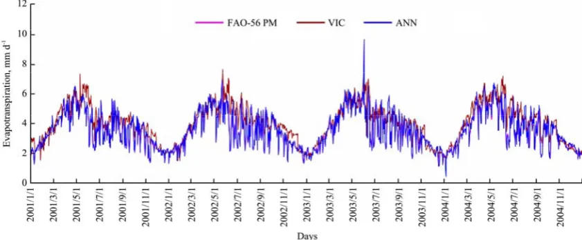
Figure 3 and 4 show the time series plots of ANN and VIC models estimated ETofor Mohanpur location during
training (2001-2004) and testing (2005), respectively with respect to FAO-56 PM ETo. This figure illustrates the
close relationship between FAO-56 PM estimated ETo
and ETo estimated from ANN models. The ANN
estimated ETo values were exactly superimposed with the
FAO-56 PM ETo estimates as compared to VIC estimated ETo values.
Figure 5a and 5b shows the scatter plots of VIC and
ANN estimated ETo with respect to FAO-56 PM,
respectively for Mohanpur location. ANN estimated ETo
agreed well with the FAO-56 PM EToand are distributed
closer to one and zero, respectively. Comparison of Figure 5a, Figure 5b revealed that the spread of ANN estimated ETo around 1:1 line was less than that of the
VIC estimated ETo. The ANN EToestimates were well
agreed with the FAO-56 PM ETovalues with high values
of R2 (= 0.998) for Mohanpur location. The above results indicated that, agreement of both the ANN and VIC models with the FAO-56 PM was good. Further, the ANN models gave a better estimation of ETo as compared
to VIC models for Mohanpur location.
Figure 3 Comparison of VIC and ANN estimated ETo with respect to FAO-56 PM ETo during training (2001-2004)
Figure 4 Comparison of VIC and ANN estimated ETo with respect to FAO-56 PM ETo during testing (2005)
a. VIC b. ANN
Figure 5 Scatter plots for comparison of VIC and ANN estimated ETo with respect to FAO-56 PM ETo during testing (2005)
4 Conclusions
ETo was estimated by VIC model by using water
balance approach which was incurred after calibration
and validation of the model. To overcome the aforementioned limitation, a methodology for indirect estimation of ETo at the watershed-scale was framed, and
macro-scale model was used. The water balance mode was selected in order to carry out the rainfall-runoff simulation for this study, in which, ETo is computed as a
water balance component. Subsequently, to test the accuracy of these ETo estimates, the results were
inter-compared with the benchmark FAO-56 PM and ANN models. Note that the past studies mostly use either the FAO-56 PM model as the base model depending on the meteorological data availability conditions. The VIC model has an advantage of taking into account the sub-grid soil moisture variability and LULC classes along with the benefit of being an open source model. Because of this reason, the VIC model was used for this study area. The ETowas estimated using two models such as VIC and
ANN. Both the models’ results were compared using three performance indices such as r, R2 and d. The results reveal that the VIC simulated ETo showed r = 0.853, R2=
0.727 and d = 0.924; while ANN models showed better agreement with r = 0.999, R2= 0.998 and d = 0.999 with the FAO-56 PM method. Hence, it is concluded that the ANN showed better results as compared to VIC model for EToestimation in Mohanpur climatic location.
References
Adamala, S., N. S. Raghuwanshi, and A. Mishra. 2015a. Generalized quadratic synaptic neural networks for ETo Modeling. Environmental Processes, 2(2): 309–329.
Adamala, S., N. S. Raghuwanshi, A. Mishra, and M. K. Tiwari. 2014a. Evapotranspiration modeling using second-order neural networks. Journal of Hydrologic Engineering,19(6): 1131–1140. Adamala, S., N. S. Raghuwanshi, A. Mishra, and M. K. Tiwari. 2014b. Development of generalized higher-order synaptic neural-based ETo Models for different agroecological regions in India. Journal of Irrigation and Drainage Engineering,
140(12): 04014038.
Adamala, S., N. S. Raghuwanshi, A. Mishra, and M. K. Tiwari. 2015b. Closure to evapotranspiration modeling using second-order neural networks. Journal of Hydrologic Engineering, 20(9): 1131–1140.
Adamala, S., N. S. Raghuwanshi, A. Mishra, and R. Singh. 2017. Generalized wavelet-neural networks for evapotranspiration
modeling in India. ISH Journal of Hydraulic Engineering, 1-13. DOI: 10.1080/09715010.2017.1327825.
Adamala, S., Y. A. Rajwade, R. Y. V. Krishna. 2016. Estimation of crop evapotranspiration using NDVI vegetation index. Journal of Applied and Natural Science, 8(1): 159–166.
Allen, R. G., L. S. Pereira, D. Raes, and M. Smith. 1998. Crop evapotranspiration: Guidelines for computing crop water requirements. Irrigation and Drainage Paper No. 56. Rome: FAO.
Billah, M. M., J. L. Goodall, U. Narayan, J. T. Reager, V. Lakshmi, and J. S. Famiglietti. 2015. A Methodology for evaluating evapotranspiration estimates at the watershed-scale using GRACE. Journal of Hydrology, 523: 574–586.
Cai, X., Z. Yang, Y. Xia, M. Huang, H. Wei, L. Leung, and M. B. Ek. 2014. Assessment of simulated water balance from NOAH, NOAH-MP, CLM, and VIC over CONUS using the NLDAS test bed. Journal of Geophysical Research: Atmospheres,
119(24): 13751–13770.
Debnath, S.,S. Adamala, and N. S.Raghuwanshi. 2015. Sensitivity analysis of FAO-56 Penman-Monteith method for different agro-ecological regions of India. Environmental Processes, 2(4): 689–704.
Kumar, M., N. S. Raghuwanshi, R. Singh, W. W. Wallender, and W. O. Pruitt. 2002. Estimating evapotranspiration using artificial neural network. Journal of Irrigation and Drainage Engineering, 128(4): 224–233.
Liang, X., D. P. Lettenmaier, E. F. Wood, and S. J. Burges. A simple hydrologically based model of land surface water and energy fluxes for General Circulation Models. Journal of Geophysical Research, 99(D7): 14415–14428.
Pai, D. S., L. Sridhar, M. Rajeevan, O. P. Sreejith, N. S. Satbhai, and B. Mukhopadhyay. 2014. Development of a new high spatial resolution (0.25×0.25) long period (1901-2010) daily gridded rainfall data set over India and its comparison with existing data sets over the region. Mausam, 65(1): 1–18. Rajeevan, M., J. Bhate, J. D. Kale, and B. Lal. 2006. High
resolution daily gridded rainfall data for the Indian region: analysis of break and active. Current Science, 91(3): 296–306. Srivastava, A., B. Sahoo, N. S. Raghuwanshi, R. Singh. 2017.
Evaluation of variable infiltration capacity model and MODIS-Terra satellite-derived grid-scale evapotranspiration in a river basin with tropical monsoon-type climatology. Journal of Irrigation and Drainage Engineering, 143(8): 04017028. Willmott, C. J. 1981. On the validation of models. Physical