NUMERICAL STUDY AND CORRELATIONS DEVELOPMENT ON TWIN-PARALLEL JETS FLOW WITH NON-EQUAL OUTLET VELOCITIES

NUMERICAL STUDY AND CORRELATIONS DEVELOPMENT ON

TWIN-PARALLEL JETS FLOW WITH NON-EQUAL OUTLET

VELOCITIES

Nidhal Hnaiena_{, Salwa Marzouk}a_{, Lioua Kolsi}a,b,*_{, Abdullah A.A.A. Al-Rashed}c_{, Habib Ben Aissia}a_{, Jacques Jay}d

a _{Unit of Metrology and Energy Systems, National Engineering School of Monastir, Monastir University, Tunisia}

b _{College of Engineering, Mechanical Engineering Department, Haïl University, Haïl City , Saudi Arabia}

c _{Dept. of Automotive and Marine Engineering Technology, College of Technological Studies, the Public Authority for Applied Education and}

Training, Kuwait

d _{Thermal Center of Lyon (CETHIL - UMR CNRS 5008), INSA Lyon, France}

A

The purpose of the present paper is to numerically investigate two plane turbulent parallel jets using CFD model. A parametric study was carried out to evaluate the simultaneous effect of the nozzle spacing and the velocity ratio on the merge point (MP), the combined points (CP) as well as the upper (UVC) and lower (LVC) vortices centers positions. Results show that the velocity ratio significantly affects twin-parallel jets flow structure. In fact, increasing the velocity ratio moves the MP, CP, UVC and LVC further upstream along the longitudinal direction while deflecting toward the stronger jet along the transverse direction. Due to the merge and combined points main role on the merging process launching and interruption, correlations predicting the merge and combined points positions are provided as a function of the nozzle spacing and the velocity ratio. These correlations are of major importance in the quick estimate of these characteristics points positions which manage two parallel jets flow in various industrial applications.

Keywords: Combined point, Merge point, Parallel jets, Nozzles spacing, Velocity ratio, Vortices centers.

1.

INTRODUCTION

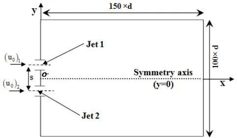
Multi-jets flows are frequently encountered in several industrial and engineering applications such as entrainment and mixing processes in boiler and gas turbine combustion chamber, injection and carburetor systems, waste disposal plums from stacks, heating and air-conditioning systems, vertical take-off and landing of air plane. In recent decades, this type of flow has attracted considerable interest of researchers. Several studies are available on multiple turbulent jets. The earliest study was that of Miller and Commings (1960) in which measurements of the mean velocity and the static pressure are carried out along the flow field of two plane parallel jets. The flow structure and entrainment mechanism in two parallel jets were investigated by Tanaka (1970 and 1974) who found that the flow field consists of three relevant regions: the converging region, the merging region and the combined region (Fig. 1). The first region, termed as the converging region is located between the nozzle exit and the point where the two jets merge. This point is called the merge point. This region is characterized by the entrainment of the surrounding fluid by turbulent jet mixing, which creates a lower pressure zone wherein is formed a reverse flow. The second zone termed the merging zone wherein the merging process between the jets occurs. This zone expands to the point where the longitudinal velocity along the flow symmetry axis is maximum, this point is called the combined point. The last zone named

* _{Corresponding author. Email: [email protected]}

the combined zone is downstream of the combined point where the whole flow behaves like a single plane jet.

Murai et al. (1976) experimentally studied two planes parallel jets flow. Measurements of pressure and stream-wise velocity were made using hot wire in the converging and combined regions while studying the nozzle converging angle effect. Marsters (1960) carried out measurements of the mean velocity and the static pressure along the flow field of two plane parallel ventilated jets. They found that the velocity profiles maintain their self-similarity behavior only in the converging and combined regions. In addition, the static pressure distribution is not affected by the Reynolds number variation for 8600≤ Re≤15700. Elbanna and Gahin (1982) experimentally investigated the merging between two parallel jets. They measured the mean velocity, the turbulence intensity and the Reynolds shear stress. By comparing their results for two parallel jets to those for a single jet, they found, in the combined zone, that the dynamic half-width for two jets changes linearly with the longitudinal distance and its propagation angle is slightly lower than that of a single jet. Elbanna and Sabbaght (1987) experimentally investigated the velocity ratio effect on the static pressure, the mean and fluctuation velocities. They found that for a velocity ratio r≠1, the weaker jet (with lower outlet velocity) is deflected towards the stronger jet (with higher outlet velocity). Lin and Sheu (1990 and 1991) have experimentally considered the nozzle spacing effect on the merge point position. Using

Frontiers in Heat and Mass Transfer

2 hot wire anemometry, Lin and Sheu (1990 and 1991) picked up the mean velocity and the Reynolds shear stress cartography. They showed that in the converging and combined zones, the mean velocity approaches self-preservation. They showed also, that the two jets spreading rate in the converging zone is greater than that of a single jet in the same region. Nasr and Lai (1997) measured the velocity fields of two plane parallel jets. They showed that for a nozzle aspect ratio (the ratio between the length and the width of the nozzle) less than 24, the side plates should be installed to improve the two-dimensionality of the flow. In addition, they found that the flow is independent of the Reynolds number for 11000 ≤ Re ≤ 19300.

Wang et al. (2001) studied analytically the incompressible multiple jet using the Prandtl mixing length hypothesis. Their results show that, in the longitudinal direction, the longitudinal velocity decreases as a single jet, while in the transverse direction, the velocity profile follows a cosine function whose amplitude decreases gradually when increasing the longitudinal distance, and finally approaches a flat profile. Two plane parallel jets are studied by Anderson and Spall (2001), experimentally using hot wire anemometry and numerically employing two turbulence models: k-ε and RSM. They compared their numerical and experimental results over a range of nozzle spacing 9 ≤ S ≤ 18.25. They found that both turbulence models could accurately predict the combined point position, but they over-predict the mean velocity distribution in the combined zone by 3 to 5%. In their work, the k-ε turbulence model shows a deviation from the experimental results. The effect of buoyancy on the merge point location is numerically studied by Spall (2002) using the experimental setup of Anderson and Spall (2001). He showed that the slight change in buoyancy has an important effect on the merge point location. Indeed, increasing buoyancy is accompanied by a decrease in the merge point longitudinal position, while for a Richardson number Ri > 0.25, Spall (2002) found that the merge point location is independent of the nozzle spacing.

The interaction between two planes parallel jets for different velocity ratio is investigated experimentally by Fujisawa et al. (2003) using PIV technique. The objective of their study was to examine the velocity ratio effect on the development of this flow in the converging zone. They found that the two parallel jets flow develops towards the side of the stronger jet and that the jet half-width is reduced when increasing the velocity ratio. It is also found that increasing the velocity ratio weakened the turbulence intensity, the Reynolds stress and the static pressure and their peaks are moved toward the side of the stronger jet. Fujisawa et al. (2003) results show that the interaction between two plane parallel jets is smaller as the velocity ratio increases. Suyambazhahan et al. (2007) numerically studied two plane parallel jets and compared their results to those experimental performed by Lin and Sheu (1990) and Spall (2002). They studied the temperature and velocity fields oscillation characteristics. The analysis is carried out for the Reynolds number 9000 ≤ Re ≤ 12000 and the Grashof number 50 ≤ Gr ≤1000. Comparison between experimental and numerical results reveals an excellent agreement concerning the merge point location and the velocity profile. They also investigated the Reynolds number, the nozzle spacing and the jet inlet temperature effect in two parallel jets flow structure.

The merging phenomenon in two and three parallel jets is numerically studied by Durve et al. (2012) using both k-ε and RSM turbulence models. The two and three jets flows simulation were respectively based on the experimental setup of Anderson and Spall (2001) and Nishimura et al. (2000). Durve et al. (2012) studied the nozzle spacing and the velocity ratio effect in the merge and combined point’s locations. They found that the merge point location depends not only on the nozzles spacing but also on the nozzles exit condition such as the turbulent intensity. Recently, Wang et al. (2016) experimentally studied two water jets flow issue from two parallel rectangular channels using two-component LDA technique. The nozzle spacing and the aspect ratio were respectively 3.1 and 15. The nozzles exit Reynolds number was approximately 9100 and the turbulent intensity was 8%. Wang et al. (2016) found that the longitudinal location of the merge point was

between X = 1.72 and X = 3.45 and that of the combined point was X = 15.52. The turbulence study showed that the outer boundary of the combined jet and the outer edges of the two jets had higher turbulence levels due to high velocity gradients in those regions. The maximum Reynolds shear stress reach its maximum at a longitudinal position of X = 5.17, which means that the flows mix stronger in some location downstream of the merge point.

Through all the studies that we have just mentioned, it appears that the majority of these works are mainly concentrated on the Reynolds number, the turbulence intensity and the nozzles spacing effect on dynamics characteristics of two plane parallel jets. However, some studies, in addition to their rarity, have focused on the velocity ratio effect on the merge and combined point’s positions. Along these works, correlations predicting the characteristic points positions are simply given in terms of a single parameter which is the nozzles spacing while two parallel jets flow is highly dependent on two parameters namely the nozzle spacing S and the velocity ratio r. To the author’s knowledge, no correlation that predicts the merge and combined point positions as a function of the nozzle spacing and the velocity ratio is found in the literature. This study aims therefore to fill these gaps. It is important to note that this is the first time that correlations predicting the merge and combined point’s longitudinal and transverse positions are given as a function of the nozzles spacing and the velocity ratio.

2.

MATHEMATICAL FORMULATION

The present simulated model which is based on the geometric configuration of Anderson and Spall (2001) for two plane parallel turbulent jets is shown in Fig. 1. Both nozzles are identical and rectangular. The width and length of each one was respectively d=6.35 mm and l = 203 mm. The turbulence intensity at the nozzles exit is I0 = 3.6% and the Reynolds number is Re=6000, which relates to a velocity initial value u0=18 m/s. The computed domain dimensions are chosen so as not to affect the flow spreading. Several configurations are tested to finally adopt the following dimensions such as 150×d and 100×d respectively along the longitudinal and transverse directions (Fig. 1). To validate our simulated numerical model, the two jets (jet 1 and jet 2) are supposed having the same initial velocity which mean that the velocity ratio considered is r = 1. On the other hand, three different nozzle spacing are used for validation such as S = 9, S = 13 and S = 18.25.

Fig. 1 Geometric configuration (Anderson and Spall (2001)) and computed domain dimension.

2.1. Hypothesis

3 and 1999) and Kriaa et al. (2002) for single free jet flow case as well as in the study of Habli et al. (2001) for single free axisymmetric jet flow. Consequently, it is possible to avoid three-dimensional (3D) calculations which are expensive in terms of time and computer hardware performance by adopting the present 2D simulation. So, 2D simulation is then sufficient to evaluate the present two parallel jets flow behavior. The work fluid is air assumed incompressible and the thermo-physical properties are constant. The jets are emitted in the longitudinal direction (along x axis). The flow is assumed to be turbulent, fully developed and supposed in a steady state.

Fig. 2 Schematic diagram of two plane parallel jets.

2.2. Governing equation

The Reynolds averaged Navier-Stoks equations can be written as follows:





0

xi



_











i

u

p ui j

u u_{i j} u u_{i j}

x_j  x_i x_j  x_j x  x_j   

  

  

 _ _

  

 



 _{ }  _   

      (2)

The additional term’’u u_{i j}  ’’ which present the turbulence effect now appear. In order to close Equation (2), this term is modeled using the following Boussinesq approximation:

u

u_{i j}

u u_{i j t}

x_j x_i

 

 

 

 

 

   

   

  (3)

Several turbulence model are tested in the present study and the k-ε model present in preliminary the best agreement with the experimental results. For this model, two additional transport equations are solved. One for the turbulent kinetic energy k and the other for the dissipation rate of the turbulent kinetic energy ε as follow:

 

i k b M k

i i k j

k

ku G G Y S

x x x

  

 _{ }  _{ } _  _{     }

  

  _  _  _

(4)

 





i 1 k 3 b 2

i i j

u C G C G C S

x x _ x k   k 

  

 _{ }  _ _ _  _{   }

  

  _ _  _

(5) In Equation (4-5), Gk represents the turbulence kinetic energy generation due to the mean velocity gradient. While Gb is the generation of turbulence kinetic energy due to buoyancy. Concerning YM, this term represents the fluctuating dilatation contribution in the compressible turbulence to the overall dissipation rate. Finally Sk and Sε are the source terms. The turbulent viscosity μt is written in terms of k and ε as follows:

2 k C t

     (6)

Solving Equations (1-6) requires the use of standard model constants provided by Hossain et al. (1982) as shown in Table 1.

Table 1. Standard k-ε model constants Constant c₁ c2 c





Value 1.44 1.92 0.09 1 1.3

2.3. Grid distribution and boundary conditions

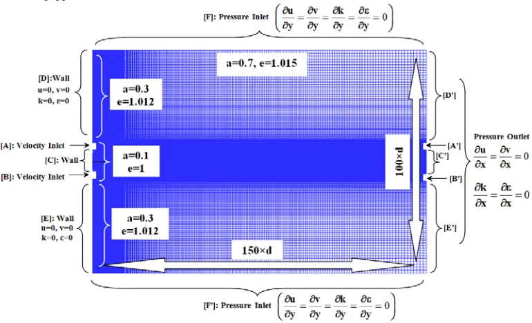
A non-uniform grid is adopted along the longitudinal and the transverse directions. Indeed, a fine grid is used near the nozzle plate and a little looser further. As shown in Fig. 3, an uniform grid is used for the [A], [B] and [C] segments with a spacing a = 0.1. The [D] and [E] segment has a non-uniform grid with spacing a = 0.3 and an expansion ratio e = 1.012 which result a nodes number of 300 on these segments ([D] and [E]).

4 Note that the grid spacing "a" is put in it dimensionless form by the nozzle width d and the expansion ratio e is a non-dimensional coefficient. For [F] segment, the grid is non-uniform with a = 0.7 and e = 1.015 which give a nodes number of 214. It is noted that all opposite segments (presented by (') symbol) have the same grid size.

Consequently we obtained a total number of quadratic cells over the entire domain as follow:





totale A B C D E F

N  N N N N N N 400 214 85600  (7)

It seems important to note that this particular choice of nodes number will be discussed later in the grid size sensitivity test section. To complete the problem, besides the equations mentioned above, it is necessary to take into account the boundary and emission conditions which are presented in Fig. 3 and detailed in Table 2.

Table 2. Boundary and emission conditions Segments Boundary _condition Details

[A] and [B] (Nozzles

outlet)

VELOCITY INLET

0

u 18m s





0 0 0

3

k I u 0.63m² s²

2   3 2 0 3 0 C k 184.8m² s 0.07d    

[C], [D] and [E] (Nozzles

plate)

WALL u0,v0,k0,0

[F] and [F']





amb

P P

u v k

0

y y y y

 _ _ _ _

   

[A'], [B'], [C'], [D'] and

[E']





PRESSURE OUTLET

amb

P P

u v k ₀

x x x x

 _ _ _ _

   

2.4. Numerical method

In this work, the transport equation associated to the boundary and emission conditions are solved numerically based on CFD code FLUENT using finite volume method developed by Pantakar (1980). The computed region is divided into finite number of sub-regions called "control volume". The resolution method is to integrate on each control volume the transport equations such as the momentum conservation, the mass conservation, the turbulence kinetic energy k and the dissipation rate of kinetic turbulence energy ε. These equations are discretized using the second order upwind. The coupling velocity-pressure is based on the SIMPLEC algorithm. The global solution convergence is obtained when the normalized residuals fall below 10-4_.

3.

RESULTS AND DISCUSSION

3.1. Velocity field validation and grid size sensitivity test

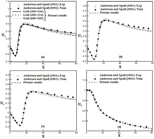
Figure 4 shows the longitudinal mean velocity evolution on the symmetry axis (y = 0) using the standard k-ε turbulence model for different nozzles spacing S = 9 (Fig. 4a), S = 13 (Fig. 4b) and S = 18.25 (Fig. 4c) as well as for single jet case (Fig. 4d). As shown in Fig. 4a, three different grids size were tested such as (300×154), (400×214) and (600×309). These grids contain respectively 46200, 85600 and 185400 quadratic cells. It is clear that the velocity profiles predicted by the grids (400×214) and (600×309) are almost identical while a remarkable difference was found between the prediction by the grids (300×154) and (400×214). Note that, the grid size (300/154) have a maximum discrepancies of 9% while the (400/214) and (600/309) grids have almost

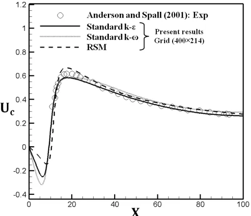
the same maximum discrepancies approximately less than 1.5% compared to Anderson and Spall (2001). Thus, the grid (400×214) is sufficient to obtain a numerical solution independent of the grid size and validated by the experimental results of Anderson and Spall (2001). It can be seen from Fig. 4 that our results (using 400×214 grid size) present good agreement with those experimental given by Anderson and Spall (2001) for the other nozzles spacing S = 13 (Fig. 4b), S=18.25 (Fig. 4c) as well as for single jet case (Fig. 4d). On the other hand, some difference is remarked between the numerical and experimental results of Anderson and Spall (2001) which shows the performance of our simulated model to give better results compared to those numerical of Anderson and Spall (2001). In Fig. 5, the same velocity profile validation is presented for nozzle spacing S = 9 using three turbulence models: standard k-ε, standard k-ω and RSM. Note that the standard k-ε model gives a better agreement with the experimental results of Anderson and Spall (2001) in the converging and combined zones. However, a slight difference is observed in the merging zone while the other two models over-predict the longitudinal velocity in the merging and combined zones.

3.2. Flow characteristic

We present in Fig. 6 the longitudinal velocity U contours (Fig. 6a), the static pressure (1000×P) contours (Fig. 6b) and the turbulent kinetic energy (1000×K) contours (Fig. 6c) along the different zone of two parallel jets flow namely the converging zone, the merging zone and the combined zone for a nozzles spacing S = 9, a Reynolds number Re = 6000 and for a velocity ratio r = 1.

Fig. 4 Longitudinal velocity profile along the symmetry axis (a) S=9, (b) S=13, (c) S=18.25, (d) Single jet.

5

Fig. 5 Turbulence models sensitivity test for the longitudinal velocity profile.

This region is characterized by a gradual increase in the longitudinal velocity (the color changes from light blue to green then yellow) (Fig. 6a), by a decrease in the static pressure (from red to yellow and green (Fig. 6b) as well as in the turbulent kinetic energy (from red to yellow and green colors) (Fig. 6c). Beyond the last point of the merging zone called the combined point (CP) where le longitudinal velocity along the symmetry axis is maximum, the flow reaches the combined zone. Along this region the two jets combine and their resulting flow behaves like a single plane jet. On the other hand, the longitudinal velocity, the static pressure and the kinetic turbulent energy decrease with the longitudinal distances and finally keep constant values.

3.3. Nozzle spacing effect on merge point (MP), combined point (CP), upper vortex center (UVC) and lower vortex center (LVC) positions

3.3.1. Upper vortex center (UVC) and lower vortex center (LVC) positions

The flow structure of two plane parallel jets is shown in Fig. 7 using streamline and velocity magnitude contours for a Reynolds number Re = 6000, a velocity ratio r = 1 and for different nozzles spacing S=6 (Fig. 7a), S = 9 (Fig. 7b) and S = 13 (Fig. 7c). This figure shows the centers of two vortices with opposite directions in the converging zone: an upper vortex (its center denoted UVC: Upper Vortex Center) on the side of the upper jet (jet 1) and another lower vortex (LVC: Lower Vortex Center) on the side the lower jet (jet 2). These vortices are also observed in previous numerical investigation on two jets flow combining an offset jet and a wall jet (Wang and Tan (2007), Kumar (2015a and b) and Hnaien et al. (2017a and b) as well as in two plane parallel jets flow (Miller and Commings(1960)).

It is clear from Fig. 7 that these vortices dimension increases when increasing the nozzle spacing S. The same observation is mentioned in the numerical simulation of Kumar (2015b) for combined wall and offset jet flow. This author noticed that more the wall jet is far away from the offset jet, more the upper and lower vortices size becomes higher. It is also clear from Fig. 7 that increasing the nozzles spacing S results in a longitudinal displacement of the UVC and LVC more downstream while transversally moving away from Y = 0 axis which present a symmetries axis for this type of flow (Fig. 7). Moreover, for all considered nozzles spacing S, the UVC and LVC remain always symmetrical with respect to y = 0 hence the name "symmetry axis" of the two parallel jets flow.

Fig. 6 Longitudinal velocity U (a), static pressure 1000×P (b) and turbulent kinetic energy 1000×K (c) contours along two parallel jet flow for Reynolds number Re = 6000, nozzles spacing S = 9 and velocity ratio r = 1.

3.3.2. Merge point (MP) and combined point (CP) positions

6

Fig. 7 Streamlines and velocity magnitude contours for Reynolds number Re = 6000, velocity ratio r = 1 and for different nozzles spacing S = 6 (a), S = 9 (b) and S = 13 (c)

Figure 8 clearly show that increasing the nozzles spacing S results in an increase in the longitudinal positions of the MP, CP, UVC and LVC. This mean that, more the upper (Jet 1) and the lower (Jet2) jets are far away from each other, more the MP, CP, UVC and LVC move downstream along the longitudinal direction. On the other hand, increasing S result in an increase of the UVC transverse position, a decrease in the LVC transverse position while the MP and CP transverse position remain equal to zero. In fact, along the transverse direction, the UVC and LVC move away from this symmetry axis (y = 0) while remaining symmetrical to y = 0 which agree well with the remarks extracted from the streamline contours (Fig. 7). On the other hand, the merge (MP) and combined (CP) points keep their positions on the symmetry axis (y = 0).

The longitudinal positions of the merge and combined points are respectively shown in Fig. 9a and b for a velocity ratio r=1 and for nozzles spacing 3 ≤ S ≤ 20, next to others previous experimental and

numerical results. Fig. 9 shows that the merge (MP) and combined (CP) points longitudinal positions increase when increasing the nozzles spacing S.

This figure shows that this increase in the longitudinal position follows a linear function and can be approximated by the following equations:

mp

X 1.01 S 0.4  (8)

cp

X 0.89 S 9.6  (9)

7 It is clear that our results are in good agreement with the majority of the studies presented in Fig. 9. A small gap is observed between our results and those of Fujisawa et al. (2003) and Nasr and Lai (1997) for the combined point position (Fig. 9b).

Fig. 9 Merge point (a) and combined point (b) longitudinal positions with respect to the nozzles spacing for a velocity ratio r = 1.

3.4. Velocity ratio effect on merge point (MP), combined point (CP), upper vortex center (UVC) and lower vortex center (LVC) positions

3.4.1. Upper vortex center (UVC) and lower vortex center (LVC) positions

Figure 10 shows the streamline and velocity magnitude contours for a Reynolds number Re = 6000, a nozzles spacing S = 9 and for different velocity ratio r = 1 (Fig. 10a), r = 1.5 (Fig. 10b) and r = 1.8 (Fig. 10c). It is clear from this figure that the upper and lower vortices sizes decrease for high velocity ratio r values . It is also noted that increasing r moves the UVC and the LVC more upstream along the longitudinal direction while deflecting towards the stronger jet (jet 1) along the transverse direction. It is also noted that for a velocity ratio r > 1 (Fig. 10b and c), the weaker jet (with lower initial velocity: Jet 2) is deviated toward the stronger jet (with higher initial velocity: Jet 1), so y = 0 axis is no longer a symmetry axis for the two parallel jet flow. Consequently, the UVC and LVC lose their symmetry with respect to y = 0 axis.

3.4.2. Merge point (MP) and combined point (CP) positions

The velocity ratio effect on the merge point (MP), the combined point (CP), the upper (UVC) and the lower (LVC) vortices centers position is evaluated in Fig. 11 with the help of the U = 0, V = 0 and dU/dY = 0

contours for the nozzle spacing S = 9 and for different velocity ratios r = 1 (Fig. 11a), r = 1.5 (Fig. 11b) and r = 1.8 (Fig. 11c). It is clear from this figure that the MP, CP, UVC and LVC positions decrease when increasing the velocity ratio r while their transverse positions increase with r. Consequently, for higher r values, these points moves more upstream along the longitudinal direction while deflecting transversally toward the stronger jet (Jet 1). Consequently, the merge and combined points are no longer located on Y=0 axis and the UVC and LVC are not any more symmetric with respect to this axis as for r=1 case.

Fig. 10 Streamlines and velocity magnitude contours for Reynolds number Re = 6000, nozzles spacing S=9 and for different velocity ratios r = 1 (a) r = 1.5 (b) and r = 1.8 (c)

3.5. Nozzles spacing and velocity ratio simultaneous effect on the merge point (MP) and combined point (CP) positions

Figures 12a and b show respectively the variation of the longitudinal Xmp and the transverse Ymp positions of the merge point (MP) with respect to the nozzle spacing S and for different velocity ratios r. The merge point’s positions and the nozzles spacing are dimensionless with the nozzle width d.

8 for different nozzle spacing, the merge point occurs always on the symmetry axis (at y = 0) as established by Anderson and Spall (2001), Lin and Sheu (1990), Tanaka (1974), Militzer (1977), Murai et al. (1976) and Miller and Commings (1960) while for r > 1, the merge point moves longitudinally further upstream and transversally deviate from the symmetry axis. This mean that, the merging process of two jets happens further upstream and the weaker jet (with lower initial velocity: jet 2) is deviated toward the stronger jet (with higher initial velocity: jet 1) which is consistent with the results established by Elbanna and Sabbaght (1987), Fujisawa et al. (2003) and Durve et al. (2012).

Fig. 11 Longitudinal velocity U = 0, transverse velocity V = 0 and dU/dY = 0 contours for Reynolds number Re = 6000, nozzle spacing S = 9 and for different velocity ratio r = 1 (a), r = 1.5 (b) and r = 1.8 (c).

This deviation phenomenon can be explained by the difference on the pressure reduction rate produced by each jet. The pressure reduction rate depends on the entrained fluid amount that in turn depends on the jet exit velocity. So, the pressure in the vicinity of the weaker jet is larger than that in the vicinity of the stronger jet. Therefore the weaker jet (jet 2) is deflected towards the stronger jet (Jet 1). From Fig. 12a, it is noted that the slope of Xmp curve as a function of the nozzles spacing S decreases for higher velocity ratio r values. Consequently, the nozzles spacing effect on the longitudinal position of the merge point is less

remarkable for r > 1. This can be explained by the fact that the transverse velocity magnitude for r > 1 is greater than that for r = 1.

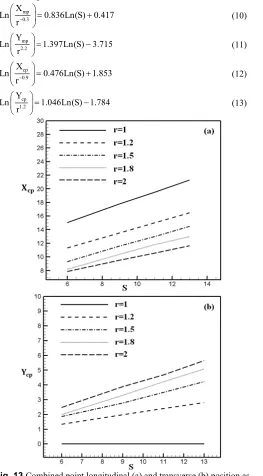
In addition, the velocity ratio r and the nozzles spacing strongly affect the combined point (CP) position. In Fig. 13, we show the velocity ratio and the nozzles spacing effect on the longitudinal Xcp and transverse Ycp positions of the combined point. This figure shows that for fixed nozzles spacing S, the longitudinal position of the combined point moves further upstream when the velocity ratio r increases while its transverse location increases with the velocity ratio. We note then, that increasing the velocity ratio promotes the appearance of the combined point more upstream along the longitudinal direction.

Fig. 12 Merge point longitudinal (a) and transverse (b) position as a function of the nozzles spacing for different velocity ratio.

3.6. Correlations development for the merge and combined points positions

Knowing the merge (MP) and the combined (CP) points positions is mandatory to have a complete idea about the lunching and interruption of the merging process in two plane parallel jets flow. As it has already been shown, these positions are strongly affected by the nozzles spacing S and the velocity ratio r. Therefore, it is desirable to determine an estimating method of the merge and combined points positions based on these important parameters (S and r).

To achieve this objective, we proposed empirical correlations that predict the dimensionless longitudinal and transverse positions of the merge and combined points. Fig. 14 presents the scatter plots relating to

mp 0.3

X Ln

r

 

 

 (Fig. 14a),

mp 2.2

Y Ln

r

 

 

 (Fig. 14b),

cp 0.9

X Ln

r

 

 

 (Fig. 14c) and

cp 1.2

Y Ln

r

 

 

 (Fig. 14d) curves as a function of Ln S for the dimensionless

 

9 and 2, these scatter plots, as shown in Fig. 14, may be approximated by the following linear functions:

mp 0.3

X

Ln 0.836Ln(S) 0.417

r

 _{ }

 

  (10)

mp 2.2

Y

Ln 1.397Ln(S) 3.715

r

 

 

 

  (11)

cp 0.9

X

Ln 0.476Ln(S) 1.853

r

 _{ }

 

  (12)

cp 1.2

Y

Ln 1.046Ln(S) 1.784 r

 

 

 

  (13)

Fig. 13 Combined point longitudinal (a) and transverse (b) position as a function of the nozzles spacing for different velocity ratio.

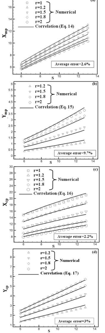
Equations (10-13) allow us to deduce correlations that attach the merge and combined points positions to S and r, these correlations are as follows:

0 3 0 836 mp

X 1 517 r . S.

. 

   6 ≤ S ≤ 13 and 1 ≤ r ≤ 2 (14)

2.2 1.397 mp

Y 0.024 r S 6 ≤ S ≤ 13 and 1 ≤ r ≤ 2 (15)

0.9 0.476 cp

X _6.379 r_  _S

6 ≤ S ≤ 13 and 1 ≤ r ≤ 2 (16)

1.2 1.046 cp

Y 0.168 r S 6 ≤ S ≤ 13 and 1 ≤ r ≤ 2 (17) Equations (14) and (16) predicted the merge and combined point’s longitudinal positions for a nozzle spacing 6 ≤ S ≤13 and a velocity ratio 1 ≤ r ≤ 2 while Eqs. (15) and (17) predict the merge and combined points transverse positions for 6 ≤ S ≤ 13 and 1.2≤r≤2 since for r=1 the merge and combined points are located on the symmetry axis for all considered nozzles spacing (Ymp = Ycp =0). The prediction of Xmp, Ymp, Xcp and Ycp respectively by Equations (14-17) next to the present numerical results is

showed in Fig. 15. It is clear from this figure that the developed correlation present a satisfactory agreement with the numerical results already showed in Figs. 12 and 13 with an average error of 2.6%, 9.7%, 2.2% and 3% respectively for Xmp, Ymp, Xcp and Ycp.

10

Fig. 15 _{Merge point (a, b) and combined points (c, d) positions given by}

Equations (14-17) compared to the numerical results.

4.

CONCLUSIONS

Turbulent multi-jets flow combining two plane parallel jets was numerically investigated using finite volume method. The discussion focuses on the standard k-ε turbulence model validity to predict the flow in three different zones. A detailed analysis is carried out to determine the nozzles spacing and the velocity ratio effect on the longitudinal and transverse positions of the merge point, the combined point and the

vortices centers. Correlations that predict the merge and combined points longitudinal and transverse positions with respect to the nozzle spacing ( 6 ≤ S ≤ 13) and the velocity ratio (1 ≤ r ≤ 2) were also provided in the present study.

The results showed that for a velocity ratio r=1, the increase in the nozzles spacing S is accompanied by a displacement of the merge point (MP), the combined point (CP), the upper vortex center (UVC) and the lower vortex center (LVC) further downstream along the longitudinal direction. This movement follows a linear function described by Eqs. (8-9) respectively for the merge and combined points. Along the transverse direction, increasing the nozzles spacing S results that the upper and lower vortices centers (UVC and LVC) move away from y=0 axis while remaining symmetrical with respect to this axis. Concerning the merge (MP) and combined (CP) points, these latter are always located on the symmetry axis (y=0) for the different considered nozzles spacing S.

On the other hand, increasing the velocity ratio (r>1) moves the MP, CP, UVC and LVC further upstream along the longitudinal direction while deflecting toward the stronger jet along the transverse direction. So the merge and combined point are no longer located on y=0 axis and the upper and lower vortices centers are no longer symmetrical with respect to y=0. For r>1, y=0 is not anymore a symmetry axis for the two parallel jets flow. It is noted that the nozzles spacing S effect on the longitudinal positions of the merge and the combined point decreases by increasing the velocity ratio while its effect on the transverse positions increase. The merge and combined points positions according to the velocity ratio r and the nozzles spacing S are described by the proposed numerical correlations (Eqs. (14-17)).

NOMENCLATURE

l Nozzle length (mm) d Nozzle width (mm)

Re Reynolds number_Reu d0



u Dimensional longitudinal velocity (m/s)

U Dimensionless longitudinal velocity

0

u U

u



p Dimensional static pressure (Pa)

P Dimensionless static pressure amb 2 0

p p P

u

 



s Dimensional nozzle spacing (mm)

S Dimensionless nozzle spacing S s d



r Velocity ratio

 

 

u r

u



x Dimensional longitudinal coordinate (mm)

X Dimensionless longitudinal coordinate X x d



y Dimensional transverse coordinate (mm)

Y Dimensionless transverse coordinate Y y d



k Dimensional turbulent kinetic energy





K Dimensionless turbulent kinetic energy ₂

0

k K

u



I Turbulence intensity (%) a Grid spacing

e Grid expansion ratio Greek symbols

11

 Kinematic viscosity





 Dynamic viscosity





 Fluid density





Subscripts 1 Jet 1 2 Jet 2

0 Initial value (at the nozzle exit) t Turbulent value

amb Ambient value Abbreviations MP Merge Point CP Combined Point UVC Upper Vortex Center LVC Lower Vortex Center

REFERENCES

Anderson, E.A. and Spall, R.E., 2001, “Experimental and Numerical Investigation of Two Dimensional Parallel Jets,” ASME J. Fluids Eng, 123, 401–406. http://dx.doi.org/10.1115/1.1363701

Durve, A. and Patwardhan, AW., 2012, “Numerical Investigation of Mixing in Parallel Jets,” Nuclear engineering and design, 242, 78-90.

https://doi.org/10.1016/j.nucengdes.2011.10.051

Elbanna, H., Gahin, S., Rashed, M.I.I., 1982, “Investigation of Two Plane Parallel Jets,” AIAA Journal, 21, 986–991.

https://doi.org/10.2514/3.8187

Elbanna, H., Sabbagh, J.A., 1987, “Interaction of Two Non-Equal Plane Jets”, AIAA Journal, 25, 12–13. https://doi.org/10.2514/3.9571

Fujisawa, N., Nakamura, K., Srinivas, K., 2003, “Interaction of Two Parallel Jets of Different Velocities,” Journal of visualization, 7, 135– 142. https://doi.org/10.1007/BF03181586

Habli, S., Mhiri, H., El Golli, S., 2001, “Etude Numérique des Conditions D’émission sur un Ecoulement de Type Axisymétrique Turbulent,” International Journal of Thermal science, 40, 497-511.

https://doi.org/10.1016/S1290-0729(01)01238-8

Hassain, M.S., Rodi, W., 1982, “A Turbulence Model for Buoyant Flows and its Application to Vertical Buoyant Jet in Turbulent Jets and Plumes,” Pergamon Press, 121-178.

https://doi.org/10.1016/B978-0-08-026492-9.50007-4

Hnaien, N., Marzouk, S., Ben Aissia, H., Jay, J., 2017, “Wall Inclination Effect in Heat Transfer Characteristics of a Combined Wall and Offset Jet Flow,” International Journal of Heat and Fluid Flow, 64, 66-78.

https://doi.org/10.1016/j.ijheatfluidflow.2017.01.010

Hnaien, N., Marzouk, S., Ben Aissia, H., Jay, J., 2017, “CFD Investigation on the Offset Ratio Effect on Thermal Characteristics of a Combined Wall and Offset Jets Flow,” Heat and Mass Transfer, 53(8), 2531–2549. https://doi.org/10.1007/s00231-017-2000-0

Kriaa, W., Mhiri, H., El Golli, S., 2002, “Etude Numérique d’un Jet Plan à Masse Volumique Variable en Régime Laminaire,”Rev. Energ. Ren, 5, 93-106.

Kumar, A., 2015, “Mean Flow Characteristics of a Turbulent Dual Jet Consisting of a Plane Wall Jet and a Parallel Offset Jet,” Computers and Fluids, 114, 48–65.

https://doi.org/10.1016/j.compfluid.2015.02.017

Kumar, A., 2015, “Mean Flow and Thermal Characteristics of a Turbulent Dual Jet Consisting of a Turbulent Wall Jet and a Parallel Offset Jet,” Numerical heat transfer Part A, 67, 1075-1096.

http://dx.doi.org/10.1080/10407782.2014.955348

Lin, Y.F., Sheu, M.J., 1990, “Investigation of Two Plane Parallel Unventilated Jets,” Experiments in Fluids, 10, 17–22.

http://dx.doi.org/10.1007/BF00187867

Lin, Y.F., Sheu, M.J., 1991, “Interaction of Parallel Turbulent Plane Jets,” AIAA Journal, 29, 1372–1373. http://dx.doi.org/10.2514/3.10749

Marsters, G.F., 1960, “Interaction of Two Plane Parallel Jets”, AIAA Journal, 15, 1756–1762.

Mhiri H., El Golli S., Le Palec G., 1998, “Influence des Conditions D’émission sur un Ecoulement de Type Jet Plan Laminaire Isotherme ou Chauffé, ”Revue Générale de Thermique, 37, 898-910.

https://doi.org/10.1016/S0035-3159(98)80014-7

Mhiri H., Habli S., El Golli S., 1999, “Etude Numérique des Conditions D’émission sur un Ecoulement de Type Jet Plan Turbulent Isotherme ou Chauffé,” International Journal of thermal science. 38, 904-915.

https://doi.org/10.1016/S1290-0729(99)80044-1

Miller D. R., Comings E.W., 1960, “Forced Momentum Fields in a Dual Jet Flow,” J. Fluid Mech. 7, 237-256.

https://doi.org/10.1017/S0022112060001468

Militzer, 1977, “Dual plane parallel turbulent jets,” Ph.D. Thesis.University of Waterloo.

Murai K., Taga M., Akagawa K., 1976, “An Experimental Study on Confluence of Two Two-Dimensional Jets”, Bulletin JSME, 19, 958.

Nasr A., Lai C.S., 1997, “Two Parallel Plane Jets: Mean Flow and Effects of Acoustic Excitation,” Experiments in Fluids, 22, 251–260.

https://doi.org/10.1007/s003480050044

Nishimura M., Tokuhiro A., Kimura N., Kamide H., 2000, “Numerical Study on Mixing of Oscillating Quasi-Planar Jets with Low Reynolds Number Turbulent Stress and Heat Flux Equation Models,” Nuclear Engineering and Design. 202, 77–95.

https://doi.org/10.1016/S0029-5493(00)00287-9

Patankar S., 1980. “Numerical Heat Transfer and Fluid Flow, Hemisphere,” New York.

Spall R.E., 2002, “Numerical Study of Buoyant Plane Parallel Jets,” ASME Journal of heat transfer, 124, 1210–1213.

https://doi.org/10.1115/1.1501088

Suyambazhahan S., Das S.K., Sundararajan T., 2007, “Numerical Study of Flow and Thermal Oscillations in Buoyant Twin Jets”, International Communications in Heat and Mass Transfer, 34, 248–258.

https://doi.org/10.1016/j.icheatmasstransfer.2006.11.006

Tanaka E., 1970, “The Interference of Two-Dimensional Parallel Jets (1st Report),” Bulletin JSME Experiments on dual jet, 13, 272–280.

http://doi.org/10.1299/jsme1958.13.272

Tanaka E., 1974, “The Interference of Two-Dimensional Parallel Jets (2nd Report),” Bulletin JSME Experiments on the combined flow of dual jet, 17, 920–927. http://doi.org/10.1299/jsme1958.17.920

Wang G.H., Priestman D.W., 2001, “An Analytical Solution for Incompressible Flow Through Parallels Multiple Jets,” ASME J. Fluids Eng, 123, 407–410. https://doi.org/10.1115/1.1363612

Wang H., Lee S., Al Hassan Y., 2016, “Laser-Doppler Measurements of The Turbulent Mixing of Two Rectangular Water Jets Impinging on a Stationary Pool,” International Journal of Heat and Mass Transfer, 92, 306-227. https://doi.org/10.1016/j.ijheatmasstransfer.2015.08.084

Wang X., Tan S., 2007, “Experimental Investigation of the Interaction between a Plane Wall Jet and a Parallel Offset Jet”, Exp. Fluids, 4, 551– 562.