R E S E A R C H
Open Access
Joint level-set and spatio-temporal
motion detection for cell segmentation
Fatima Boukari and Sokratis Makrogiannis
*FromIEEE International Conference on Bioinformatics and Biomedicine 2015 Washington, DC, USA. 9-12 November 2015
Abstract
Background: Cell segmentation is a critical step for quantification and monitoring of cell cycle progression, cell migration, and growth control to investigate cellular immune response, embryonic development, tumorigenesis, and drug effects on live cells in time-lapse microscopy images.
Methods: In this study, we propose a joint spatio-temporal diffusion and region-based level-set optimization approach for moving cell segmentation. Moving regions are initially detected in each set of three consecutive sequence images by numerically solving a system of coupled spatio-temporal partial differential equations. In order to standardize intensities of each frame, we apply a histogram transformation approach to match the pixel intensities of each processed frame with an intensity distribution model learned from all frames of the sequence during the training stage. After the spatio-temporal diffusion stage is completed, we compute the edge map by nonparametric density estimation using Parzen kernels. This process is followed by watershed-based segmentation and moving cell detection. We use this result as an initial level-set function to evolve the cell boundaries, refine the delineation, and optimize the final segmentation result.
Results: We applied this method to several datasets of fluorescence microscopy images with varying levels of difficulty with respect to cell density, resolution, contrast, and signal-to-noise ratio. We compared the results with those produced by Chan and Vese segmentation, a temporally linked level-set technique, and nonlinear diffusion-based segmentation. We validated all segmentation techniques against reference masks provided by the international Cell Tracking Challenge consortium. The proposed approach delineated cells with an average Dice similarity coefficient of 89 % over a variety of simulated and real fluorescent image sequences. It yielded average improvements of 11 % in segmentation accuracy compared to both strictly spatial and temporally linked Chan-Vese techniques, and 4 % compared to the nonlinear spatio-temporal diffusion method.
Conclusions: Despite the wide variation in cell shape, density, mitotic events, and image quality among the datasets, our proposed method produced promising segmentation results. These results indicate the efficiency and robustness of this method especially for mitotic events and low SNR imaging, enabling the application of subsequent
quantification tasks.
Keywords: Cell segmentation, Level sets, Nonlinear diffusion, Density estimation
*Correspondence: [email protected]
Department of Physics and Engineering, Delaware State Univ., 1200 N. DuPont Hwy, Dover, DE 19901, USA
Background
Cell identification, quantification and characterization using imaging techniques are emerging research areas that are systematically integrated in biological and med-ical studies [1]. Recent developments in time-lapse microscopy enable the observation and quantification of cell-cycle progression, cell migration, and growth control [2]. The tasks of detecting and tracking individual cells or particles in a time series of images are key elements in this process. More importantly, the large volume of data pro-duced by fluorescence microscopy and imaging modalities emphasizes the need for automated and robust techniques that can address the challenges in accurate detection and segmentation as well as tracking.
Cell tracking methodologies involve the tasks of pre-processing, cell segmentation and motion tracking [3–9]. In this context, segmentation of cells is a particularly challenging task that has a direct impact on the overall quantification process. Image segmentation is a popular field in the domain of image analysis. More specifically, parametric [10] and nonparametric active contour models [11–14] have been widely used in development of bio-imaging and biomedical image analysis techniques. An interesting aspect in cell analysis methods is the relation between image quality and segmentation accuracy. Many segmentation methods address certain types of datasets; however, for low-quality images and different cell types and shapes, the same methods may yield varying levels of performance.
Earlier published works propose to use partial differ-ential equation (PDE) models for heat diffusion to detect motion with applications to moving edge detection [15], and human assistive technologies [16]. Building upon previous ideas for estimating motion activity using spatio-temporal diffusion [16], in this work we develop and uti-lize a heat flow analogy model in the joint spatio-temporal domain and combine this process with a region-based level-set optimization approach for cell segmentation of images obtained by fluorescence microscopy. Spatial and temporal motion parameters of our model are estimated for each dataset and an optimal Parzen bandwidth param-eter is experimentally dparam-etermined for density estimation of edges and outliers in each dataset. High activity regions are initially detected by solving numerically a system of coupled spatio-temporal nonlinear partial differential dif-fusion equations on three consecutive frames. In order to obtain more stability in parameter choice, we apply a histogram transformation approach to match the refer-ence background threshold from the intensity distribution of each three consecutive frames to an intensity distribu-tion model learned from all frames of the sequence during the training stage. After this step, each video sequence frame is scaled and transformed into a sequence with background with same order of magnitude for a more
robust and a less sensitive parameter choice method. Then spatial and temporal motion parameters of our model are estimated for each dataset and an optimal Parzen bandwidth parameter is experimentally estimated for den-sity estimation for edges and outliers for each dataset. After the spatio-temporal diffusion stage is completed, we compute the edge map by nonparametric density esti-mation using Parzen kernels. This process is followed by watershed-based segmentation to detect the moving cells. Next, adjacent regions with motion are merged to form a moving cell by mean intensity thresholding of these regions. Thresholding determines the boundary of each cell. Finally, the moving delineation curve is used as an initial level-set to be refined using a region-based process for final segmentation. We validated the joint approach denoted by ST-Diff-TCV over a set of sequences against reference data and compared the segmentation accuracy of the joint spatio-temporal and level-set tech-nique with results derived from Chan-Vese (CV) segmen-tation [17], a temporally linked level set method that we have recently presented [18] denoted by TCV, and spatio-temporal diffusion based segmentation only (ST-Diff ). Our method can accurately detect fluorescent cells at an average Dice coefficient rate of 89 % showing a clear improvement over region-based level set segmen-tation with and without temporal linking, and nonlinear diffusion-based segmentation. In addition, it can detect and segment newly appearing cells. Another feature of this method is it can detect cells hardly detectable by means of mean intensity and produces accurate results for high or low cell density images. This method allows to detect cells that were impossible to detect using the region based CV segmentation because the optimization criterion is defined by the mean intensity inside and out-side the level set defined moving curve. Hence, cell regions with low intensity values are considered as part of the background, and the region competition process fails to delineate these cells. However, these regions are detected by the spatio-temporal motion detection method because they are rather detected by their high activity process than by their intensity value, then refined by CV model to detect the cell boundaries more accurately.
CV, TCV, ST-Diff, and ST-Diff-TCV, followed by discus-sion of results. Finally, in the concludiscus-sion we summarize the main observations about the advantages of this method and perspectives for future work.
Methods
Frame intensity standardization by histogram transformation
PDE-based techniques calculate differential approxima-tions; therefore they are sensitive to variations in pixel intensity ranges. The main objective of this stage is first to reduce intensity variations between frames of each sequence, and second, to obtain a robust intensity prior for the cell delineation process. We apply a histogram transformation approach to match the intensity distribu-tion of each three consecutive frames defined by (1) to an intensity distribution model learned from all frames of the sequence during the training stage.
P3F(I)= lim Ntotal→∞
N(I) Ntotal
, F3F(k)=
k
0
P3F(I)dI (1)
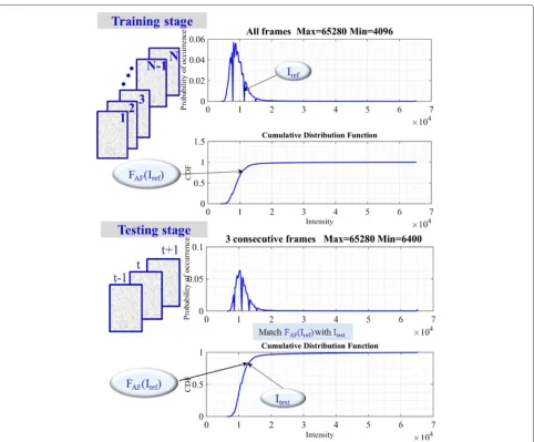
The general idea is to transform the frame intensities so that the reference cell/background thresholdIref deter-mined from theFAFas expressed in (2) matches the global CDF referenceFAF(Iref)corresponding to theIref value (2) indicating the tail of background intensity distribution of the complete sequence as displayed in Fig. 1 (top).
PAF(I)= lim Ntotal→∞
N(I) Ntotal
, FAF(k)=
k
0
PAF(I)dI
(2)
We aim to find a transformation so that the output image is a similar image that has a background value with the same order of brightness of the input image. Figure 1 (bottom) displays how we can determine the Itest value from the PDF of each three consecutive frames at the training stage using the prior valueFAF(Iref)as expressed by (3).
Itest=argmin
i |F3F(I(ω))−FAF(Iref)|, (3)
whereω ∈ 3F, I : Z2 → R+. Using these values, the resulting images are scaled and defined over the [0−255] range and with respect to the global minimum and global maximum intensities of all the frames of the dataset sequence after applying Eqs. 4, (5) and (6).
T1(I)=
Iref −GMin Itest−LMin(
I−GMin)+GMin (4)
T2(I)=
255·(I−GMin) GMax−GMin
(5)
IS(ω)=T(I(ω))=(T2◦T1)(I(ω)), ω∈3F (6)
We experimentally found that the matched frames are less sensitive to the temporal, spatial diffusion parameters and Parzen kernel bandwidth values than the raw frames. In our experiments we used 256 bins for all datasets.
The following steps define the two algorithms that learn the CDF reference value for background intensity FAF(Iref)at the training stage (Algorithm 1) and transform every source image at the testing stage (Algorithm 2) so as to make its testing background as close as possible to the reference intensity.
Algorithm 1Histogram transform training stage
Require: datasetD= {D1,D2,. . .,DN}
1: DAF←ConcatenateDk, k=1,. . .,N
2: GlobalMax←Maximum pixel intensity ofDAF
3: GlobalMin←Minimum pixel intensity ofDAF
4: PlotPAF(I)=limNtotal→∞
N(I)
Ntotal
5: Choose (reference value)Iref inPAF at beginning of histogram tail for background distribution
6: FAF(k)← k
0PAF(I)dI
7: FAF(Iref)←Closest percentile ofIref
8: return FAF(Iref),GlobalMax,GlobalMin,Iref,
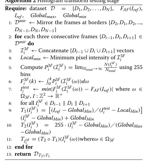
Algorithm 2Histogram transform testing stage
Require: dataset D = {D1,D2,. . .,DN}, FAF(Iref), Iref, Globalmax, Globalmin
1: Dmir ←Mirror the frames at borders{D2,D1,D2, ...,
DN−1,DN,DN−1}
2: foreach three consecutive frames{Di−1,Di,Di+1} ∈ Dmirdo
3: Ii3F ←Concatenate{Di−1∪Di∪Di+1}vectors 4: Localmin←Minimum pixel intensity ofIi3F
5: ComputePi3F(Ii3F) = limNtotal→∞
N(Ii3F)
Ntotal using 255
bins
6: Fi3F(k)←0kPi3F(Ii3F(ω))dω
7: Iitest ← min|Fi3F(Ii3F(ω))−FAF(Iref)| whereω ∈ 3F,I:Z2→R+
8: for allIi3F∈Di−1DiDi+1 9: T1(I3iF) =
(Iref −GlobalMin)(Iitest−LocalMin)
(Ii3F−GlobalMin)+GlobalMin
10: T2(I3iF) = 255·(Ii3F−GlobalMin)(GlobalMax −GlobalMin)
11: TI3F
i =(T2◦T1)(I 3F
i (ω))whereω∈3F
12: end for 13: return DT2◦T1
Fig. 1(Training stage) Probability density function of 48 frames of C2DL−MSC02 dataset and cumulative distribution function. (Testing stage) Normalized PDF and CDF of three consecutive frames of C2DL−MSC02 dataset
transformations T1 andT2 given by (4) and (5)
respec-tively. The bottom row shows the histogram of 3 frames used to determine Itest, the original histogram of cur-rently processed frame and transformed histogram after applying (6).
We note that after the histogram transformation and scaling, all frames of the same sequence are going to have similar pixel intensity ranges.
Spatio-temporal diffusion Perona-Malik anisotropic diffusion
Diffusion algorithms perform image restoration by find-ing numerical solutions of the heat diffusion PDE [19, 20]. In this framework, the linear diffusion model is equiva-lent to applying Gaussian filtering to the image. To avoid the blurring and localization problems of linear diffusion filtering, Perona and Malik [21] proposed to replace the
classic isotropic diffusion equation with the nonlinear diffusion model, which is based on the following PDE:
∂I ∂s =div
g(|∇I(x,y,s)|)· ∇I(x,y,s) (7)
whereIis the image intensity,sthe scale variable for 2D case, and g(·) a function that determines the amount of diffusion, also known as diffusivity function. This function is chosen to satisfy limx→∞g(x) → 0 so that
diffu-sion is attenuated across edges. This function controls the amount of diffusion according to the edgestrength. Common options forg(·)are the sigmoid and exponential functions also reported by Perona and Malik in [21]:
g(x)= 1 1+xk22
Fig. 2Histogram of all concatenated images of the C2DL-MSC02 dataset, and linear transformations and scaling of each pixel of the image (top row, left to right). The histogram of three consecutive frames that will be matched to the training dataset, and the histograms of the current frame before and after the transformationT(I(ω))=(T2◦T1)(I(ω)), ω∈3F(bottom row, left to right)
g(x)=e
−x2 k2
(9)
where k denotes the conductance parameter that is a positive constant. The anisotropic diffusion method has been extensively used for image restoration as it largely preserves edge image features.
Moving regions are initially detected in each three consecutive frames by numerically solving the spatio-temporal partial-differential diffusion equation [18] where the diffusivity function is applied to the gradient magni-tude of the imageI. In this work we used the function (9) that is more suitable for region oriented applications [22]. This nonlinear diffusion is bound to the gradient magni-tude [23]. It applies more diffusion in uniform regions and slows down at edges, therefore preserves high contrast edges over low contrast ones.
Spatio-temporal nonlinear diffusion
Partial differential equation model Here we propose to simulate nonlinear heat flow through the processed frames in both spatial and temporal dimensions. This operation smooths-out the background regions and simultaneously preserves the spatio-temporal discontinuities corresponding to cells. More specifically,
given 3 consecutive frames of the sequence at times {t−1,t,t+1}, we define a system of three coupled PDEs for each frame.
At time pointsτ = {t−1,t,t+1}
∂I(i,j,τ,s)
∂s =g(|∇I(i,j,τ,s)|)·I(i,j,τ,s) + ∇g(|∇I(i,j,τ,s)|)· ∇I(i,j,τ,s)
(10)
Initial condition
I(i,j,τ, 0)=I0(i,j,τ) (11)
Boundary condition
∂I
∂n =0 on∂×∂T×(0,S). (12)
At t
Iis,+j,t1=Iis,j,t+λs
g|∇Iis+1,j,t|·Nt+g
|∇Iis−1,j,t|·St + g|∇Iis,j+1,t|·Et+g
|∇Iis,j−1,t|·Wt +λt
∇Iis,j,t−1·PF+ ∇Iis,j,t+1·NF (13)
At t−1
Iis,+j,t1−1=Iis,j,t−1+λs
g
|∇Iis+1,j,t−1|
·Nt−1 +g|∇Iis−1,j,t−1|·St−1 +g
|∇Iis,j+1,t−1|
·Et−1 +g
|∇Iis,j−1,t−1|
·Wt−1 −2λtPF· ∇Iis,j,t−1·PF
(14)
At t+1
Iis,+j,t1+1=Iis,j,t+1+λs
g|∇Iis+1,j,t+1|·Nt+1 +g|∇Iis−1,j,t+1|·St+1 +g
|∇Iis,j+1,t+1|
·Et+1 +g|∇Iis,j−1,t+1|·Wt+1 −2λtNF· ∇Iis,j,t+1·NF
(15)
where
Nt=Isi−1,j,t−Iis,j,t, St=Iis+1,j,t−Iis,j,t (16)
Wt=Iis,j−1,t−Iis,j,t, Et=Iis,j+1,t−Iis,j,t (17)
PF=Iis,j,t−1−Iis,j,t, NF=Iis,j,t+1−Iis,j,t (18) In (13), (14), and (15) λs, λt, λtPF, λtNF denote the numerical “time” steps for spatial, temporal, next frame temporal, and previous frame temporal terms respec-tively. In our implementation we set λt = TSRatio ·λs andλtPF = λtNF, whereTSRatio is a fixed parameter for the ratio of temporal to spatial diffusion. The diffusiv-ity function is applied to the gradient magnitude of the imageI.
Detection of spatio-temporal discontinuities by Parzen density estimation
The idea is to estimate the likelihood of mean inten-sity in the neighborhood of each pixel in the diffused frame. Assuming a model of unimodal probability den-sity function (PDF) for region interiors and bimodal PDF for edges, we use the likelihood of mean intensity as an
index of edge occurrence. Low values of this index corre-spond to a bimodal PDF indicating an edge. We estimate this likelihood by the nonparametric technique of Parzen kernels [24–26].
The Parzen density estimation belongs to the nonpara-metric density methods [23] i.e. methods to estimate the probability density function of a random variable that do not impose any initial assumptions about the shape of the probability density functions. Its operation is based on placing at each observation sample a probability mass and producing a potential according to a Gaussian kernel. The contributions of all the sample points are averaged to esti-mate the density value at every point of the image [25].
fh(x)=1/(n·hp) n
i=1
K((x−xi)/h) (19)
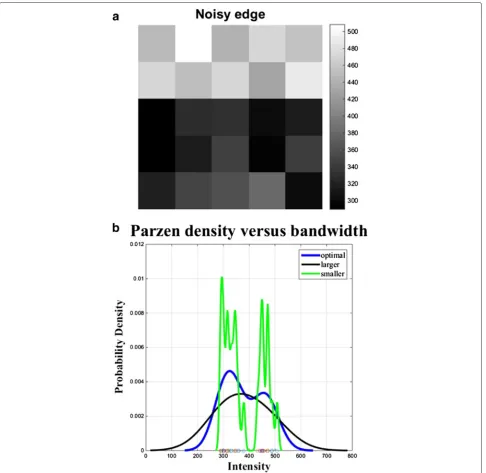
where(x1,x2, ,xn)is an independent and identically dis-tributed sample drawn from some distribution with an unknown density P, K(·) is the kernel and h > 0 is a smoothing parameter called the bandwidth. We can see in (19) that the kernel-bandwidth h can strongly affect the PDF estimate, especially when the number of observa-tionsnis finite. Very smallhvalues will produce a ragged density estimate, while very large values will smooth the structure of the PDF. An optimalhvalue is usually exper-imentally determined to find a compromise between the variability and accuracy and converge towards the true PDF. Figure 3 shows three density estimates: the green solid line corresponds to a small bandwidth, the black line corresponds to a large bandwidth, while the blue line represents a bandwidth selection that produces a more accurate estimate of the underlying bimodal distribution.
Cell delineation and identification
Fig. 3An example ofanoisy edge detection usingbnonparametric density estimation. Comparison of the Parzen density estimate for different bandwidth values ofhon the same image intensity samples plotted on the horizontal axis. The optimalhvalue estimates the bimodality of the local intensity distribution. Use of smallerhis susceptible to statistical variability, while largerhwill reduce the estimation accuracy
estimation to form regions separated by spatio-temporal discontinuities.
To separate the cells we calculate intensities and areas of watershed regions and classify them into cells or back-ground using area and intensity prior information and likelihoods p(area|ci), p(I|ci) in Gaussian form, where ci = {background,cell}. Adjacent watershed regions with coherent motion should be merged together to form a moving object. We compute mean intensity over the
watershed regions and classify into foreground or back-ground using as threshold value the standardized refer-ence valueT(Iref)calculated by (6).
of region-based statistics may prove advantageous for images characterized by edge discontinuity and higher level of noise. Chan-Vese (CV) method [17] is a region-based active contour model for energy minimization. Here, we shortly describe the theoretical background of Chan-Vese model and its minimization framework. This model is a special case of the Mumford-Shah functional [28] for segmentation using piecewise constant approxi-mation.
This model segments an input scalar imageI(x,y)with I : → Rand (x,y) ∈ ⊂ R2 into two discon-nected regions 1 and 2 representing the foreground
and background respectively of low intra-region variance and separated by a smooth closed contour C such that =1∪2∪C. Chan and Vese proposed to use
level-set functions to solve this optimization problem. In the level-set method, the contour is represented as the zero level-set of a Lipschitz functionφ : → R, whereφ is positive insideCand negative outsideC. Segmentation is obtained by minimizing the following energy functional in terms of level-set:
F(φ,c1,c2)=μ·length{φ=0} +v·area{φ≥0}
+λ1
φ≥0
|I−c1|2dxdy
+λ2
φ<0|
I−c2|2dxdy
(20)
where C is the evolving curve, c1 and c2 are the
aver-age intensity levels inside and outside the contourC, and μ,ν,λ1,λ2≥0 are energy weights. The length and area of
Care regularizing terms are formulated using the Heavi-sideHand Diracδ functions. In [17] the Euler-Lagrange equations and the gradient-descent method were used to derive the following evolution equation for the level-set functionφthat minimizes the fitting energy using time to parametrize the gradient descent:
∂φ(t,x,y)
∂t =δ(φ(x,y))·
μ·div
∇φ(x,y) |∇φ(x,y)|
−v
−λ1(I−c1)2+λ2(I−c2)2 ∈(0,∞)×
(21)
with initial and Neumann boundary conditions
φ(0,x,y)=φ0(x,y)∈ (22)
δ(φ) |∇φ|·
∂φ
∂n =0∈∂ (23)
Temporally linked level-set segmentation
This approach makes use of temporal connection between consecutive level-set results [17]. That is, when segment-ing an image, which is a part of a temporal sequence, we
Algorithm 3Temporally linked Chan-Vese segmentation
Require: frame Di, curve C of spatio-temporal mask resultRSTM
1: φ0←Initial level-set signed distance(C) 2: repeat
3: Each iterationnUpdate average intensitesc1andc2 4: c1(φn) ← Mean intensity of image pixels of Di
inside the contourCn
5: c2(φn) ← Mean intensity of image pixels of Di outside the contourCn
6: F(φn,c1,c2)←Normalized energy of imageDi
7: Solve PDE ∂φ(∂tt,x,y) = 0 inφnto obtainφn+1from (21) withc1(φn)andc2(φn)
8: Reinitializeφlocally to the signed distance function
to the curve
9: untilConvergence orn>nmax
10: Apply morphological operations to the segmented
regions
11: RS←Thresholdingφfinal
12: return Binary maskRS
make use of the level-set results reached from minimiza-tion of the global energy associated with the contours of the segmented cells found in the previous time point
φn+1(x,y; 0)=φn(x,y;ifinal),∀(x,y)∈, (24) wherenis the frame number in the time-lapse sequence, andifinalis the number of iterations required to converge for frame n. We take the contour result of each frame as the initial contour for the following one. These results are utilized to minimize the energy functional of the next image. If the segmentation in framenis accurate, then this initialization will correspond to a point close to the global optimum of the energy functional in framen+1. The main steps of this technique are summarized in Algorithm 3.
Joint spatio-temporal diffusion and temporally linked level-set approach (ST-Diff-TCV)
We propose a joint method combining the S-T differen-tial information with the high delineation accuracy that characterizes level set-based segmentation [15, 17]. More specifically, we use S-T Diffusion to delineate the cells first, then initialize TCV with the S-T Diffusion result to refine the cell segmentation. We apply the S-T Diffusion technique on each modulokframe to address cell events that may not be handled by TCV such as cell mitosis, cell division, new cells entering the field of view, and other cases.
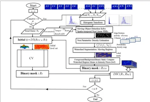
difficulty with respect to cell density, resolution, contrast, and signal-to-noise ratio. The flowchart in Fig. 4 outlines the main stages of our proposed technique. Furthermore, in Fig. 5 we display intermediate results from each stage on a test frame and its temporal neighbors for the C2DL-MSC02 and N2DH-SIM04 sequences.
Results and discussion Data description
The datasets consist of 2D fluorescent microscope time-lapse image sequences. We used 12 time-time-lapse video sequences; 6 real microscopy time-lapse sequences and 6 computer simulated videos with various cell densities and noise levels. We obtained the training and chal-lenge data sets from the cell tracking chalchal-lenge web-site [29]. Simulated videos: The 6 simulated videos displayed fluorescently labeled nuclei of the HL60 (human promyelocytic leukemia) cell line migrating on a flat 2D surface (N2DH-SIM01, N2DH-SIM02, N2DH-SIM03, N2DH-SIM04, N2DH-SIM05, N2DH-SIM06). They differ in the level of noise, cell density of the initial popula-tion, the number of cells leaving and entering the field of
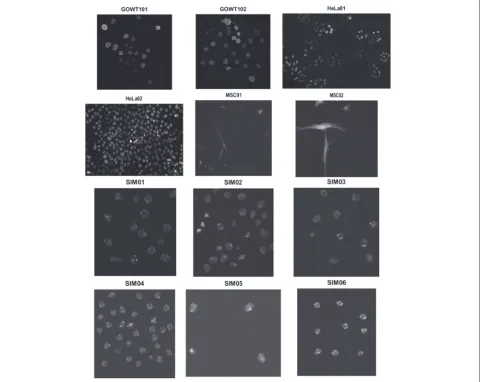
view and the number of simulated mitotic events, yield-ing up to 70 cells in the field of view [29]. Real videos: We used 3 datasets each containing 2 time-lapse sequences. Two video sequences named Fluo-C2DL-MSC01 and Fluo-C2DL-MSC02 with rat mesenchymal stem cells, 2 video sequences named GOWT101 and N2DH-GOWT102 of mouse embryonic stem cells and N2DL-HeLa01 and N2DL-HeLa02 expressing HeLa cells. These datasets are considered to have high level of difficulty [29] because of the high cell density and low resolution and intensity. Summarized information on our test data is listed in Table 1, including the image matrix size, num-ber of frames and level of difficulty. Furthermore, a sample frame of each dataset is displayed in Fig. 6.
Image quality assessment of the datasets
In our first experiment, we measured the image qual-ity of our datasets and then evaluated the segmentation accuracy. We utilized the available reference data for this purpose. The reference data consist of manually anno-tated videos for segmentation and tracking along with a short description and links to the raw datasets obtained
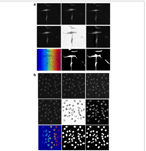
Fig. 5Intermediate results produced by ST-Diff-TCV on sample frames ofaC2DL-MSC02 andbN2DH-SIM04 data sequences.First row: center, previous and next frames in the temporal space (left to right)Second row: S-T diffused frame, kernel density estimation of edge-moving regions then the inverted probability density map.Third row: watershed result, cell identification after foreground/background separation, and the reference segmentation mask (left to right)
from [29]. We first used the reference data to estimate the average Signal-to-Noise Ratio (SNR) and Contrast-to-Noise Ratio (CNR) of each dataset. The SNR andCNR measures are defined as follows:
SNR=20 log10u¯C ¯ uB
(25)
CNR= |¯uC− ¯uB| σB
(26)
Table 1Image sequence properties and quality using Signal-to-Noise Ratio (SNR) and Contrast-to-Noise Ratio (CNR)
Dataset name Average SNR std Average CNR std Level of difficulty
N2DH-SIM01 21.53±0.69 7.96±0.95
N2DH-SIM02 22.21±0.65 8.35±0.96 Medium:different noise levels
N2DH-SIM03 18.59±0.47 4.21±0.47 cell density of the initial
N2DH-SIM04 18.97±0.47 4.09±0.49 population and number of
N2DH-SIM05 19.49±0.54 4.22±0.60 simulated mitotic events.
N2DH-SIM06 21.92±0.54 7.90±0.78
C2DL-MSC01 14.67±0.67 2.11±0.36 High:low SNR, cell strectching appear
C2DL-MSC02 15.09±2.31 4.47±1.49 as discontinuous extensions of the cells.
N2DL-HeLa01 26.60±3.41 19.23±7.67 High:high cell density, low resolution,
N2DL-HeLa02 16.02±1.67 5.40±1.08 frequent mitoses (normal and abnormal).
N2DH-GOWT101 22.47±0.49 12.62±0.77 Medium:heterogeneous staining, prominent nuclei,
N2DH-GOWT102 18.91±0.92 8.32±0.91 mitoses, cells entering and leaving the field of view
CNRthat are means over all frames in each sequence using (25) and (26) and corresponding standard deviations of each dataset over cell regions. A comparison between the qualitative level of difficulty and the image quality met-rics in Table 1 shows that the simulated sequences have higherSNRandCNR, therefore being more amenable to segmentation than the real sequences.
Comparison of CV, TCV, ST-Diff, and ST-Diff-TCV methods We applied the standard CV, TCV, ST-Diff, and ST-Diff-TCV methods on 12 time-lapse fluorescent microscopy datasets listed in Table 1. Fluorescent microscopy imag-ing is often times subjected to a mixture of different types of noise. The main goal of a preprocessing step is to reduce the corruption caused by noise and to improve the image quality [28]. To facilitate data analysis, a combina-tion of filters and histogram enhancement is applied to the datasets to obtain better delineation accuracy.
We segmented each dataset using each method and evaluated the segmentation performance against refer-ence masks. The main purpose is to evaluate how well the segmented cells match the cell regions of the refer-ence mask. We quantify the accuracy of the segmentation performance by computing the DICE similarity coefficient denoted byDSC. This is defined as:
DSC=2× |RS∩RRef| |RS| + |RRef| ∈
[0, 1] , (27)
whereRRef is the set of all pixels that belong to cell regions in the reference image,RSis the set of all binary regions delineated by the tested segmentation technique. The DICE coefficient measures the relative similarity between two binary images over their cardinalities. It is frequently used for image segmentation validation. The value of 1 indicates perfect matching.
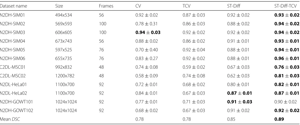
We computed the DICE coefficient between the auto-mated and reference segmentations for each method and for each dataset. Further, we computed the means and the standard deviations of the DICE similarity coefficients over all frames for each dataset sequence. Figure 7 and Table 2 report theDSCestimates and their variations for each sequence. In addition, the last row in Table 2 lists the overallDSCvalues for all datasets. In Fig. 7 and Table 2 we observe that ST-Diff-TCV yields higherDSCvalues for 11 out of the 12 test sequences. ST-Diff-TCV yields an aver-age Dice coefficient of 0.89 over all datasets, while both CV and TCV yield 0.78, and ST-Diff yields 0.85 (Table 2). Furthermore, the standard deviation values in Table 2 show more robustness and stability. That is, the stan-dard deviations obtained from ST-Diff and ST-Diff-TCV (0.01-0.03) are significantly smaller than those derived from the CV method (0.01-0.4) and even TCV (0.02-0.08) indicating better convergence and stability.
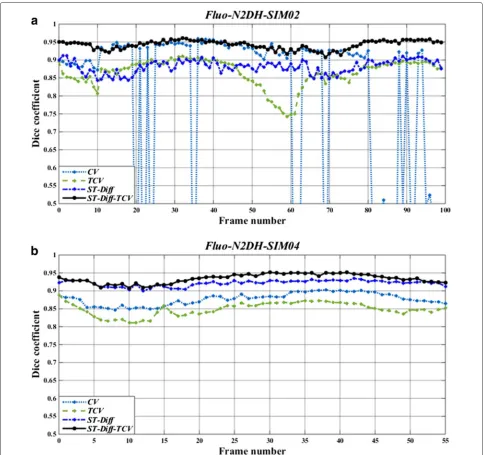
To illustrate the performance comparison among the three tested methods in more detail, we show in Fig. 8 the results derived from CV, TCV, ST-Diff, and ST-Diff-TCV methods on N2DH-SIM02 and N2DH-SIM04 datasets. In the N2DH-SIM02 sequence (Fig. 8(a)) we observe that because of the non-convexity of the energy functional (allowing therefore many local minima), the CV method reached several local minima of energy. In contrast, the TCV method led to a global minimum of the energy. ST-Diff-TCV method yields accurate delineation of the cells with fewer fluctuations in the Dice coefficient than the other methods. We note that ST-Diff-TCV yields an average Dice coefficient of 0.94, while CV yields 0.78, TCV yields 0.86, and ST-Diff yields 0.88. In the N2DH-SIM04 dataset as displayed in Fig. 8(b) we observe that ST-Diff-TCV produces the highest accuracy at aDSCvalue of 0.93, followed by ST-Diff, CV and TCV with Dice coefficients of 0.91, 0.88 and 0.86 respectively.
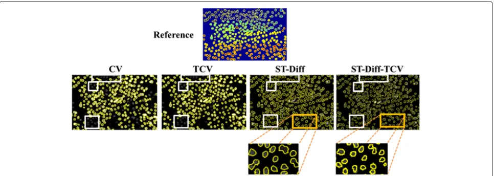
Furthermore, Fig. 9 displays cell delineations repre-sented by yellow contour maps for one frame of the sequence N2DL-Hela2 including the manual reference, and automated segmentation produced by all tested methods. This sequence has an increased level of diffi-culty because of the high cell density and low contrast between some cells and the background. Because CV and TCV methods use piecewise constant approximations for object and background as can be seen in (21), the low contrast cells are likely to be falsely identified as background therefore reducing DSC (CV: 0.84, TCV: 0.67). On the other hand, both ST-Diff and ST-Diff-TCV identify the spatio-temporal discontinuities and detect the cells that are missed by CT and TCV as outlined by white rectangles in Fig. 9. In the magnified local regions of the test image we note that ST-Diff-TCV yields more accurate cell separation for adjacent cells than ST-Diff.
Fig. 7Dice similarity coefficients (DSC) produced by standard Chan−Vese model (CV), temporally linked Chan−Vese technique (TCV), spatio−temporal diffusion (ST−Diff), and the joint ST−Diff−TCV methods over all 12 datasets
On the other hand, the proposed technique involves some motion diffusion – i.e.,TSRatio,λt, and Parzen ker-nel parameters – which are experimentally determined for each sequence. ST-Diff-TCV performance exhibits mod-erate sensitivity to the parameter values. In this work we performed exhaustive grid search in the parameter space to identify the optimal settings. Alternate parameter opti-mization techniques may be required to achieve more accurate segmentation in sequences with significantly dif-ferent quality levels and cell types. In summary, our experiments suggest that the joint ST-Diff-TCV method improves the segmentation accuracy compared to CV, TCV, and ST-Diff, especially when applied to simulated
and real microscopy images with cells characterized by wide intensity variations and undergoing mitotic events, changes in density, and lowSNR.
Conclusions
In this work, we introduced a local-global co-operative approach to dynamic cell segmentation. One com-ponent of this approach performs nonlinear spatio-temporal diffusion-based motion analysis, Parzen kernel-based detection of discontinuities, and watershed-kernel-based foreground-background separation. This local-based seg-mentation part generates a delineation that we use as the initial level-set in a region-based temporally linked
Table 2The mean DICE coefficient obtained from segmentation of each sequence by CV, TCV, ST-Diff, and the joint ST-Diff-TCV method
Dataset name Size Frames CV TCV ST-Diff ST-Diff-TCV
N2DH-SIM01 494x534 56 0.92±0.02 0.87±0.03 0.92±0.02 0.93±0.02
N2DH-SIM02 569x593 100 0.78±0.31 0.86±0.03 0.88±0.02 0.94±0.02
N2DH-SIM03 606x605 100 0.94±0.03 0.92±0.02 0.92±0.02 0.94±0.02
N2DH-SIM04 673x743 56 0.88±0.02 0.86±0.02 0.91±0.01 0.93±0.01
N2DH-SIM05 597x525 76 0.70±0.40 0.92±0.04 0.88±0.01 0.94±0.01
N2DH-SIM06 655x735 76 0.83±0.27 0.92±0.02 0.88±0.01 0.96±0.01
C2DL-MSC01 992x832 48 0.74±0.08 0.59±0.02 0.67±0.03 0.76±0.03
C2DL-MSC02 1200x782 48 0.58±0.09 0.74±0.08 0.62±0.03 0.81±0.03
N2DL-HeLa01 1100x700 92 0.72±0.01 0.68±0.02 0.80±0.01 0.82±0.01
N2DL-HeLa02 1100x700 92 0.84±0.01 0.67±0.03 0.87±0.01 0.87±0.01
N2DH-GOWT101 1024x1024 92 0.77±0.01 0.71±0.03 0.91±0.03 0.90±0.02
N2DH-GOWT102 1024x1024 92 0.68±0.02 0.67±0.03 0.91±0.02 0.92±0.02
MeanDSC 0.78 0.78 0.85 0.89
Fig. 8Dice similarity coefficients (DSC) produced by standard Chan-Vese segmentation (CV), temporally linked Chan-Vese technique (TCV), spatio-temporal diffusion (ST-Diff), and the joint ST-Diff-TCV methods for each frame ofaN2DH-SIM02 andbN2DH-SIM04 datasets
level-set model. The improvement in segmentation accu-racy is mainly achieved by using both the local motion and the global statistical information for segmenting cells with heterogeneous intensity levels. We evaluated the per-formance of our approach denoted by ST-Diff-TCV, two level-set based methods denoted by CV and TCV, and ST-Diff methods on datasets obtained from the online Cell Tracking challenge [29]. Every dataset addresses a different type of challenge for segmentation.
In comparison to CV and TCV, both ST-Diff and ST-Diff-TCV perform more robust cell segmentation,
Fig. 9Cell boundaries produced by the 4 tested methods on N2DL-HeLa02 sequence frame. The spatio-temporal analysis enables the identification of more moving cells than the level-set models. Furthermore, ST-Diff-TCV produces more accurate cell separation than ST-Diff (magnified regions)
Acknowledgements
We acknowledge the support by the Center for Research and Education in Optical Sciences and Applications (CREOSA) in Delaware State University funded by NSF CREST HRD-1242067. Research reported in this publication was also supported by the National Institute of General Medical Sciences of the National Institutes of Health under Award Number SC3GM113754. The content is solely the responsibility of the authors and does not necessarily represent the official views of the National Institutes of Health.
Declarations
This article has been published as part ofBMC Medical GenomicsVol 9 Suppl 2 2016: Selected articles from the IEEE International Conference on
Bioinformatics and Biomedicine 2015: medical genomics. The full contents of the supplement are available online at http://bmcmedgenomics.
biomedcentral.com/articles/supplements/volume-9-supplement-2.
Funding
Publication charges for this article have been funded by the National Institutes of Health.
Availability of data and materials
The time-lapse microscopy videos and the reference datasets used in this paper are publicly available by the organizers of the cell tracking challenge at http://www.codesolorzano.com/celltrackingchallenge/Cell_Tracking_ Challenge/Datasets.html.
Authors’ contributions
FB: Designed and implemented the algorithm, designed and performed validation experiments, interpreted the results and wrote the manuscript. SM: Contributed to designing and implementing the algorithm, designing the validation experiments, interpreting the results, and writing the manuscript. Both authors read and approved the final manuscript.
Competing interests
The authors declare that they have no competing interests.
Consent for publication
Not applicable.
Ethics approval and consent to participate
The experimental procedures involving human subjects and animal models described in this paper were approved by the Institutional Review Board and the Institutional Animal Care and Ethics Committee of the institutions that provided the data.
Published: 10 August 2016
References
1. Eils R, Athale C. Computational imaging in cell biology. J Cell Biol. 2003;161(3):477–81. doi:10.1083/jcb.200302097.
2. Stephens DJ, Allan VJ. Light microscopy techniques for live cell imaging. Science. 2003;300(5616):82–6. doi:10.1126/science.1082160.
3. Yang X, Li H, Zhou X. Nuclei segmentation using marker-controlled watershed, tracking using mean-shift, and kalman filter in time-lapse microscopy. Circ. Syst. I: Regular Papers IEEE Trans. 2006;53(11):2405–14. doi:10.1109/TCSI.2006.884469.
4. Zhou X, Li F, Yan J, Wong STC. A novel cell segmentation method and cell phase identification using markov model. IEEE Trans Inf Technol Biomed. 2009;13(2):152–7. doi:10.1109/TITB.2008.2007098. 5. Li F, Zhou X, Ma J, Wong STC. Multiple nuclei tracking using integer
programming for quantitative cancer cell cycle analysis. IEEE Trans Med Imaging. 2010;29(1):96–105. doi:10.1109/TMI.2009.2027813.
6. Meijering E, Dzyubachyk O, Smal I. Methods for cell and particle tracking. Methods Enzymol. 2012;504:183–200.
doi:10.1016/B978-0-12-391857-4.00009-4.
7. Chen C, Wang W, Ozolek JA, Rohde GK. A flexible and robust approach for segmenting cell nuclei from 2d microscopy images using supervised learning and template matching. Cytom Part A. 2013;83A(5):495–507. doi:10.1002/cyto.a.22280.
8. Maska M, Ulman V, Svoboda D, Matula P, Matula P, Ederra C, Urbiola A, Espana T, Venkatesan S, Balak DMW, Karas P, Bolckova T, Streitova M, Carthel C, Coraluppi S, Harder N, Rohr K, Magnusson KEG, Jalden J, Blau HM, Dzyubachyk O, Kizek P, Hagen GM, Pastor-Escuredo D,
Jimenez-Carretero D, Ledesma-Carbayo MJ, Munoz-Barrutia A, Meijering E, Kozubek M, Ortiz-de-Solorzano C. A benchmark for comparison of cell tracking algorithms. Bioinformatics. 2014;30(11):1609–17.
doi:10.1093/bioinformatics/btu080.
9. Faure E, Savy T, Rizzi B, Melani C, Stasova O, Fabreges D, Spir R, Hammons M, Cunderlik R, Recher G, Lombardot B, Duloquin L, Colin I, Kollar J, Desnoulez S, Affaticati P, Maury B, Boyreau A, Nief JY, Calvat P, Vernier P, Frain M, Lutfalla G, Kergosien Y, Suret P, Remesikova M, Doursat R, Sarti A, Mikula K, Peyrieras N, Bourgine P. A workflow to process 3d+time microscopy images of developing organisms and reconstruct their cell lineage. Nat Commun. 2016;7. doi:10.1038/ncomms9674. 10. Kass M, Witkin A, Terzopoulos D. Snakes: Active contour models. Int J
Comput Vis. 1988;1(4):321–31. doi:10.1007/BF00133570. 11. Malladi R, Sethian JA, Vemuri BC. Shape modeling with front
propagation: a level set approach. IEEE Trans Pattern Anal Mach Intell. 1995;17:158–75. doi:10.1109/34.368173.
12. Cremers D, Rousson M, Deriche R. A review of statistical approaches to level set segmentation: Integrating color, texture, motion and shape. Int J Comput Vis. 2006;72(2):195–215.
microscopy. IEEE Trans Med Imaging. 2010;29(3):852–67. doi:10.1109/TMI.2009.2038693.
14. Nath SK, Palaniappan K, Bunyak F. Cell Segmentation Using Coupled Level Sets and Graph-Vertex Coloring In: Larsen R, Nielsen M, Sporring J, editors. Medical Image Computing and Computer-Assisted Intervention – MICCAI 2006: 9th International Conference, Copenhagen, Denmark, October 1-6, 2006. Proceedings, Part I. Berlin, Heidelberg: Springer; 2006. p. 101–8.
15. Direkoglu C, Nixon MS. Moving-edge detection via heat flow analogy. Pattern Recogn Lett. 2011;32(2):270–9. doi:10.1016/j.patrec.2010.08.012. 16. Makrogiannis SK, Bourbakis NG. Motion analysis with application to
assistive vision technology. In: 16th IEEE International Conference On Tools with Artificial Intelligence, 2004. Piscataway, New Jersey: IEEE; 2004. p. 344–52. doi:10.1109/ICTAI.2004.89.
17. Chan TF, Vese LA. Active contours without edges. Image Process IEEE Trans Image Process. 2001;10(2):266–77. doi:10.1109/83.902291. 18. Boukari F, Makrogiannis S. Spatio-temporal level-set based cell
segmentation in time-lapse image sequences In: Bebis G, Boyle R, Parvin B, Koracin D, McMahan R, Jerald J, Zhang H, Drucker S, Kambhamettu C, El Choubassi M, Deng Z, Carlson M, editors. Advances in Visual Computing. Lecture Notes in Computer Science, vol. 8888. Cham, Switzerland: Springer International; 2014. p. 41–50.
19. Weickert J. Anisotropic Diffusion in Image Processing. ECMI Series. Stuttgart: Teubner; 1998. http://www.mia.uni-saarland.de/weickert/book. html.
20. Black MJ, Sapiro G, Marimont DH, Heeger D. Robust anisotropic diffusion. IEEE Trans Image Process. 1998;7(3):421–32. doi:10.1109/83.661192. 21. Perona P, Malik J. Scale-space and edge detection using anisotropic
diffusion. Pattern Anal Mach Intell IEEE Trans. 1990;12(7):629–39. doi:10.1109/34.56205.
22. You YL, Xu W, Tannenbaum A, Kaveh M. Behavioral analysis of anisotropic diffusion in image processing. IEEE Trans. Image Process. 1996;5(11):1539–53. doi:10.1109/83.541424.
23. Tsiotsios C, Petrou M. On the choice of the parameters for anisotropic diffusion in image processing. Pattern Recognit. 2013;46(5):1369–81. doi:10.1016/j.patcog.2012.11.012.
24. Parzen E. On estimation of a probability density function and mode. Ann Math Stat. 1962;33(3):1065–76.
25. Izenman A. Recent developments in nonparametric density estimation. J Am Stat Assoc. 1991;86:205–24.
26. Comaniciu D, Meer P. Mean shift: A robust approach toward feature space analysis. IEEE Trans Pattern Anal Mach Intell. 2002;24(5):603–19. doi:10.1109/34.1000236.
27. Soille P. Morphological image analysis: principles and applications, 2nd edn. Secaucus, NJ, USA: Springer; 2003.
28. Mumford D, Shah J. Optimal approximations by piecewise smooth functions and associated variational problems. Comm Pure Appl Math. 1989;42(5):577–685. doi:10.1002/cpa.3160420503.
29. Cell Tracking Challenge. 2013. http://www.grand-challenge.org/.
• We accept pre-submission inquiries
• Our selector tool helps you to find the most relevant journal
• We provide round the clock customer support
• Convenient online submission
• Thorough peer review
• Inclusion in PubMed and all major indexing services
• Maximum visibility for your research
Submit your manuscript at www.biomedcentral.com/submit