https://doi.org/10.5194/essd-9-435-2017 © Author(s) 2017. This work is distributed under the Creative Commons Attribution 3.0 License.
High-resolution elevation mapping of the McMurdo Dry
Valleys, Antarctica, and surrounding regions
Andrew G. Fountain1, Juan C. Fernandez-Diaz2, Maciej Obryk1, Joseph Levy3, Michael Gooseff4, David J. Van Horn5, Paul Morin6, and Ramesh Shrestha2
1Department of Geology Portland State University, Portland, OR 97201, USA
2National Center for Airborne Laser Mapping, University of Houston, Houston, TX 77204, USA 3University of Texas, Institute for Geophysics, Jackson School of Geosciences, Austin, TX 78758, USA
4Institute of Arctic & Alpine Research, University of Colorado, CO Boulder, 80309 5Department of Biology, University of New Mexico, Albuquerque, NM 87131, USA
6Polar Geospatial Center, University of Minnesota, St. Paul, MN 55108, USA
Correspondence to:Andrew G. Fountain ([email protected])
Received: 8 December 2016 – Discussion started: 5 January 2017 Revised: 27 May 2017 – Accepted: 29 May 2017 – Published: 12 July 2017
Abstract. We present detailed surface elevation measurements for the McMurdo Dry Valleys, Antarctica de-rived from aerial lidar surveys flown in the austral summer of 2014–2015 as part of an effort to understand geomorphic changes over the past decade. Lidar return density varied from 2 to > 10 returns m−2with an aver-age of about 5 returns m−2. Vertical and horizontal accuracies are estimated to be 7 and 3 cm, respectively. In addition to our intended targets, other ad hoc regions were also surveyed including the Pegasus flight facility and two regions on Ross Island, McMurdo Station, Scott Base (and surroundings), and the coastal margin between Cape Royds and Cape Evans. These data are included in this report and data release. The combined data are freely available at https://doi.org/10.5069/G9D50JX3.
1 Introduction
The McMurdo Dry Valleys (MDV) are a polar desert lo-cated along the Ross Sea coast of East Antarctica (∼77.5◦S, ∼162.5◦E; Fig. 1). These valleys are not covered by the East Antarctic ice sheet due to the blockage to flow by the Transantarctic Mountains and the severe rain shadow caused by these mountains (Chinn, 1981; Fountain et al., 2010). The valleys are a mosaic of gravelly sandy soil, glaciers, ice-covered lakes, and ephemeral melt streams that flow from the glaciers. Permafrost is ubiquitous, with active layers up to 75 cm deep (Bockheim et al., 2007). This region is of in-terest to geologists and biologists. It is one of the few re-gions in Antarctica with exposed bedrock from which the tectonic history of the continent can be explored (Gleadow and Fitzgerald, 1987; Marsh, 2004). The bare landscape also provides evidence for past glaciations, a critical look into the past behavior of the Antarctic Ice Sheet (Brook et al., 1993;
Denton and Hughes, 2000; Hall et al., 2010). The cold dry environment of the MDV hosts an unusual terrestrial habi-tat dominated by microbial life (Adams et al., 2006; Cary et al., 2010) and serves as a useful terrestrial analogue for Martian conditions (Kounaves et al., 2010; Levy et al., 2008; Samarkin et al., 2010).
436 A. G. Fountain et al.: McMurdo Dry Valley lidar
Figure 1. Landsat image mosaic of Antarctica, LIMA (Bind-schadler et al., 2008), map of the central McMurdo Dry Valleys with locations of UNAVCO fixed Global Positioning System ground sta-tions.
have observed glacier thinning where significant sediment deposits have collected on the surface (Fountain et al., 2014). Common to all changes is the occurrence of a relatively thin veneer of sediment over massive ice. In the case of the valley floor the sediment veneer is ∼10−1m in thick-ness, whereas on the glaciers it is patchy, with thicknesses of ∼10−3 to 10−2m. In addition, anecdotal observations point to large changes in other stream channels and increas-ing roughness and perhaps thinnincreas-ing of the lower elevations of some glaciers.
To assess the magnitude and spatial distribution of land-scape changes, the valleys were surveyed using a high-resolution airborne topographic lidar during the austral sum-mer of 2014–2015 and the results were compared to an ear-lier survey flown in the summer of 2001–2002 (Csatho et al., 2005; Schenk et al., 2004). Our working hypothesis is that landscape change is limited to the coastal thaw zone where maximum summer temperatures exceed−5◦C (Fountain et al., 2014; Marchant and Head, 2007). Here we summarize the field campaign of 2014–2015, data processing, and the point cloud of elevation data covering about 3300 km2of the MDV, and 264 km2of areas of interest nearby, all of which have been made openly available to the research community.
2 Approach
In early December 2014, the lidar personnel from the Na-tional Science Foundation’s NaNa-tional Center for Airborne Laser Mapping (NCALM) and the science team from Port-land State University arrived at McMurdo Station for an 8-week field season. Two airborne laser scanner (ALS) instru-ments were used in the survey. The main instrument was the Titan multiwave (MW), a newly designed multispec-tral ALS based on performance specifications provided by NCALM, with an integrated digital camera manufactured for
NCALM by Teledyne Optech, Inc., Toronto, Canada. It is the first operational ALS designed to perform mapping us-ing three different wavelengths simultaneously through the same scanning mechanism (Fernandez-Diaz et al., 2016a, b). Two wavelengths are in the near-infrared spectrum (1550 and 1064 nm) and the third is in the visible spectrum (532 nm). This three-wavelength capability enables the Titan MW to map elevations of solid ground (topography) and depths be-low water surface (bathymetry – but not available for reasons described later) simultaneously. This three-channel spectral information can be combined into false-color laser backscat-ter images, which improves the ability to distinguish between types of land cover. The system is mounted under the aircraft, scanning side to side at an angle of up to±30◦off nadir, pro-ducing a sawtooth ground pattern. There are 1064 nm chan-nel points at nadir and 1550 and 532 nm chanchan-nel point 3.5 and 7◦ forward of nadir, respectively. Each channel can ac-quire up to 300 000 measurements per second. However, the nominal operation pulse repetition rate for the MDV survey was 100 kHz per channel. For some extreme regions where the terrain relief was extremely high, the Titan MW had to be operated at lower pulse rates of 75 and 50 kHz. For each pulse the Titan only records first, second, third, and last re-turns. The Titan scanner was operated at an angle of±30◦ and a frequency of 20 Hz.
The advantage of Titan MW over traditional ALS sys-tems for mapping regions like the MDV where areas of soil and snow overlap is the multiple channels at different wavelengths. A traditional ALS operating at 1550 nm obtains strong returns from the soil surfaces but may have difficulties over ice and snow, which reflect less at that wavelength. The additional 1064 and 532 nm channels have a better response to snow. Also, three channels collecting data simultaneously increases the data density compared to single-channel units. However, a limitation of the Titan system is the maximum range of∼ ≤2 km.
The second ALS was an Optech Gemini airborne laser ter-rain mapper (ALTM), which served as a backup to the Ti-tan MW. The Gemini ALTM is a single-channel system that uses 1064 nm laser pulses at repetition frequencies of 33 to 166 kHz and it can scan a swath of up to ±25◦ off nadir. While the return densities obtained with the Gemini are lower than those from the Titan MW system, it has the advantage of a longer maximum range of∼ ≤4 km. The Gemini was operated at pulse rate frequency between 70 and 100 kHz, its scanner ran at±25◦and a frequency of 35 Hz; its beam divergence was set at 0.25 milliradians.
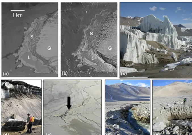
Figure 2.Examples of ice-mediated elevation changes in the McMurdo Dry Valleys. Disintegration of the lower ablation zone of the Wright Lower Glacier, Wright Valley,(a)1980 and(b)2008. S is the sediment-covered part of the glacier, G is the relatively clean part of the glacier, and L is Lake Brownworth. The dots just below the S in the 2008 photo are ice spires several meters tall with sediment-covered ablated ice surrounding it, depicted in(c), photo: M. Sharp.(d)Ice cliff exposed by the eroding Garwood River.(e)Aerial view of Garwood River incision and bank collapse. River flows right to left. Arrow points to where photos(f)and(g)were taken.(f)Recent incision; note color differences.(g)The river has carved a thermokarst tunnel.
physical chip size of 5.39 cm×4.04 cm. The image is formed on the focal plane through a compound lens with a focal length of 70 mm. The combination of lens and CCD array yields a total field of view (FOV) of 42.1◦×32.2◦ and a ground sample distance of 0.0000825×flight height (∼5 cm for nominal mission altitudes of 600 m above ground level). The position of the CCD is adjusted during flight through a piezo actuator to compensate for the motion of the aircraft during an exposure, reducing pixel smear.
To derive accurate differential kinematic trajectories for the ALS, a total of nine UNAVCO Global Positioning System (GPS) stations were used as reference, recording data at a rate of 1 Hz (Fig. 1). This network of GPS stations provided sufficient coverage to ensure that the aircraft was no more than 40 km from any station during mapping operations.
3 Results from the field campaign
The Titan MW ALS was mounted within a DHC-6 Twin Ot-ter aircraft operated by Kenn Borek Air of Calgary, Canada, under contract to the National Science Foundation. The air-craft flew at a nominal speed of 65–70 m s−1 at a nominal flight height of 600 m above the surface (actual flight heights above terrain ranged between 400 and 2500 m). The footprint of the laser beam was about 0.3 m for channels 1 and 2 and about 0.6 m for channel 3 (Fig. 3).
Figure 3.Image of the Titan channel 3 (532 nm) laser footprint captured by the digital camera over the floor of Wright Valley.
oppor-438 A. G. Fountain et al.: McMurdo Dry Valley lidar
Figure 4.Flight lines for the new 2014–2015 survey (shown in red) over the extent of the 2001 survey (shown in purple) digital eleva-tion model hillshades. Base map is the Landsat Image Mosaic of Antarctica (Bindschadler et al., 2008).
tunity were surveyed, including McMurdo Station and sur-roundings, Pegasus Airfield, and the coastal area between and including Cape Royds and Cape Evans. These ad hoc re-gions, together with the MDV, totaled about 3600 km2from which 3564 km2of elevation rasters of surveyed landscape was produced (Fig. 4).
Reliability of the Titan MW system was good, with only 1 day lost due to an intermittent malfunction. A total of 109 aircraft engine-on hours was used. Of these, 94.7 h were flying hours, which yielded a total of 50.9 laser-on hours (47.4 h with Titan MW and 3.4 h with Gemini). A total of 42.5 billion laser shots were fired, of which about two-thirds (28.7 billion) produced usable returns. The unusable returns were primarily due to a saturation of channel 3 (532 nm) of the Titan system. This channel is optimized for weak returns to enhance the ability to see through clear water (bathymetry). However, the detector was overwhelmed by sunlight reflections off the steep valley walls and multipath reflections produced by the highly reflective snow and ice. This caused the detector to trigger spurious returns, saturat-ing the ability of the sensor to record actual surface returns. The remaining usable returns were equally divided between channels 1 and 2. Returns from the outer 5◦of either side of the swath (scan angle cutoff) were also discarded to reduce scan line artifacts.
Survey patterns were described as “mowing the lawn” as the plane flew back and forth along the longitudinal axis of each valley, with the goal of 50 % overlap with the prior swath such that the edge of the newly acquired swath over-laps from the edge to the center of the adjacent previously flown swath. The separation between the flight lines was ∼350 m. Due to adverse weather 50 % lateral swath overlap was not always possible.
After the aircraft landed, preliminary processing was per-formed to examine the coverage and identify gaps to be
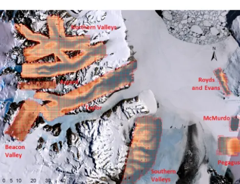
re-Figure 5.Return density map for the 2013–2014 lidar survey of the McMurdo Dry Valleys. The units of density are returns m−2×10. Base map is the Landsat Image Mosaic of Antarctica (Bindschadler et al., 2008).
flown. The time between initial and final coverage depended on weather. While the performance of Titan MW met most of its design parameters, it was not able to detect usable returns in the deeper parts of Taylor Valley because the safe flight height above local terrain exceeded the range limit of the strument. To survey these regions, the Gemini sensor was in-stalled towards the end of the flying season and the data gaps were closed. The resulting spatial point density of the laser returns varied due to differences in flight height, weather, and repeat coverage to close gaps (Fig. 5). Overall, the range of unfiltered laser returns varied from 2 to > 10 returns m−2, with an average of 4.7 returns m−2.
4 Final data processing
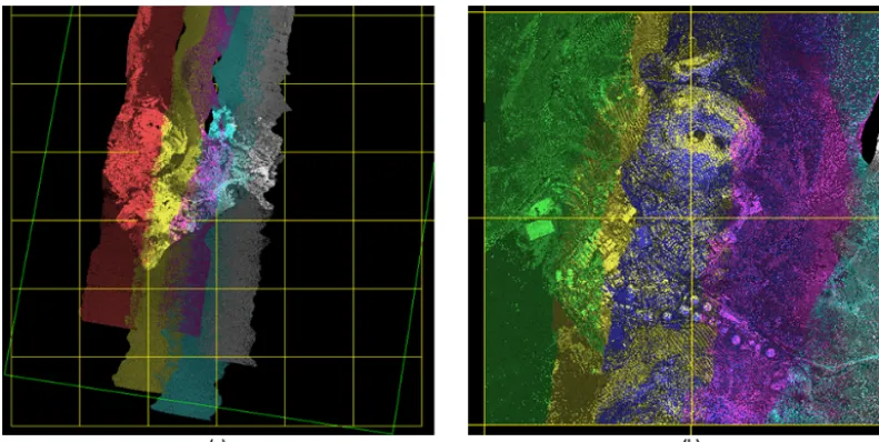
Figure 6.Lidar point cloud strips and point cloud tiles illustrating how a large coverage area is broken down into tiles.(a)Five flight strips over McMurdo Station; the strip point clouds have been rendered based on flight line and intensity. The yellow grid represents the 1 km×1 km tiles into which the returns from the different strips will be binned.(b)Point clouds for four tiles. The tiled point clouds are rendered based on flight line and intensity. The overlap between the different flight strips within each tile is evident on this rendering.
GPS stations using the KARS (Kinematic and Rapid Static) software (Mader, 1996), taking data from one GPS station at a time. For each flight its final trajectory in three dimensions was derived by blending solutions from at least three GPS stations. These data were then combined with orientation in-formation collected from the inertial measurement unit, op-erating at 200 kHz. We used a Kalman filter algorithm within POSPac Mobile Mapping Suite version 7.1 (Applanix Cor-poration) to combine these data. The final navigation solution obtained is known as a smoothed best estimated trajectory (SBET) and resulted in a binary file containing the sensor’s position and orientation.
The second processing step, point cloud production, com-bined the laser range data with the SBET to produce geo-located point clouds of laser returns. The point cloud duction was performed with the sensor manufacturer’s pro-prietary software LMS for the Titan MW and DASHmap for the Gemini. Before producing the point cloud for the en-tire project area, a small subset of the cloud was carefully examined. This geographical subset was selected before the data were collected to serve as a calibration and validation (CAL/VAL) site. The CAL/VAL site has structural and to-pographic features that allowed for the verification that all systematic sources of error that can affect the geometric and geolocation quality of the returns were accounted for. The calibration or boresight adjustment of an ALS ensured that returns were consistent with each other (within same and different flight lines) and reduced data artifacts. The point clouds obtained for the CAL/VAL area were visually and an-alytically checked and parameters were adjusted to improve the geometric quality of the returns when the point cloud was regenerated. Through this iterative process the
calibra-tion was refined to obtain a final set of calibracalibra-tion parameters that were applied to the range data for the entire project to produce the point clouds of each flight line. Each data return was positioned in three-dimensional space by horizontal co-ordinates in US Geological Survey Transantarctic Mountains Projection (epsg projection 3294) and vertical coordinate in meters above the World Geodetic Survey 1984 (WGS84) el-lipsoid.
In addition to the geolocation information, each return contains information regarding the strength of the backscat-tered energy (intensity) and the GPS time for the emission of the laser pulse. The point clouds are encoded following the American Society of Photogrammetry and Remote Sensing (ASPRS) LAS 1.2 laser return file format (.las). The point clouds produced for each flight line are referred to as strips (Fig. 6a). Because of the complexity of some strips, their size, and overlap with adjacent strips, the strips were com-bined and the coverage re-organized into orthogonal tiles of dimension 1 km×1 km, as illustrated in Fig. 6, for simplicity in handling and further processing.
440 A. G. Fountain et al.: McMurdo Dry Valley lidar
Figure 7.Illustration of assessing uncertainty for airborne lidar sur-vey (ALS) compared to terrestrial lidar sursur-vey (TLS) of an inclined roof.
line. In addition to ensuring consistency between elevations of different flight lines, this process can be tied to control points with well-known elevations such that the adjusted ele-vations are also consistent with a given vertical datum. After adjusting for these vertical offsets, the final point cloud tiles were produced. Of the 28.7 billion adequate returns from the MDV, about 50 % were discarded due to the±5◦swath edge cutoff and to noise removal, resulting in a total of 14.1 billion returns in the final point clouds.
The accuracy of the geolocation of the laser returns was verified against terrestrial laser scanning (TLS) data of build-ings and structures from McMurdo Station, which were col-lected by Merrick and Company. Planar building roofs were selected as reference. A plane was fitted to the TLS data of a roof using the linear least squares method, and the difference in elevation (dz) and perpendicular distance to plane were computed for respective airborne returns for the same planar roof surfaces (Fig. 7). The advantage of this method over the traditional methods of collecting kinematic GPS measure-ments over flat uniform surfaces such as roads and runways (Heidemann, 2014) is that it permits decomposition of the accuracy in both horizontal and vertical components. A to-tal of 35 planes were employed for the accuracy assessment, consisting of almost 560 000 TLS measurements and a total of 5008 airborne lidar returns.
The RMSE for the distance-to-plane measurement was 7.6 cm, with a vertical and horizontal component RMSE of 6.9 and 3.2 cm, respectively. It is important to make two critical observations regarding these values. First, this method might provide higher RMSE values than the tradi-tional method because the geolocation of the TLS dataset has positional uncertainties higher than a vehicle kinematic survey, which is generally used as a reference dataset for the traditional method. Second, the horizontal uncertainty is probably an underestimate, and while it represents an average value under constrained conditions (low airplane dynamics,
Figure 8.Shaded relief maps of the McMurdo Dry Valleys based on aerial lidar surveys conducted from December to January 2014– 2015. A is the northern valleys of Victoria, Barwick, McKelvey, and Wright with adjacent valleys; B is Beacon Valley and surround-ings; C is Taylor Valley and surroundsurround-ings; and D is the southern Dry Valleys of Garwood, Miers, Marshall, and adjacent valleys. E is a section of the Asgard ranges, F is Pegasus Airfield, G is the Mc-Murdo Station area, and H is Capes Royds and Evans. Base map is the Landsat Image Mosaic of Antarctica (Bindschadler et al., 2008).
600 m range), the horizontal uncertainty can be as high as 20–30 cm under more unfavorable flight conditions.
With the finalized point clouds, irregularly spaced data were interpolated, using Kriging methods, to a regularly spaced grid at 1 m intervals, forming digital elevation mod-els (DEMs). The algorithm was applied to each tile and in-cluded returns 10 m into the neighboring tiles to avoid tile boundary artifact. The tiles were mosaicked into large cov-erage rasters (∼400 km2) and converted into ArcGIS eleva-tion rasters. The gridding, mosaicking, and conversion of the DEMs was performed using Surfer software (Golden Soft-ware, Golden, CO). The ArcGIS elevation rasters were used to produce shaded relief images of the valley images with standard illumination parameters: Azimuth 315◦, elevation 45◦, andZfactor 1 (Fig. 8).
5 Data products
Table 1.Summary of available lidar data products. Returns are the lidar returns from the Earth’s surface; no. of LAS tiles is the number of point cloud tiles for each section; LAS Gb is the data storage size in gigabytes for the point cloud data; no. of sections is the number of individual sections that constitute the entire elevation raster for each region; DEM Gb is the data storage size in gigabytes of the digital elevation model that covers that region; SRM Gb is the data storage size in gigabytes of the shaded relief maps.
Region Coverage area km2 Point cloud products Elevation rasters
Returns×106 No. of LAS tiles LAS Gb No. of sections DEM Gb SRM Gb Taylor 852.8 4112.5 944 107.0 3 6.8 1.0 Northern 1289.8 5417.2 1447 141.0 3 10.1 1.6 Southern 755.1 2800.7 827 73.0 2 5.5 0.9 Beacon Valley 316.1 651.4 376 16.9 1 3.1 0.4 Asgard Range 94.8 129.5 136 3.4 1 0.7 0.1 Pegasus 157.8 504.3 181 13.1 1 0.9 0.1
McMurdo 42.3 257.9 59 6.7 1 0.3 0.1
Royds & Evans 63.4 253.3 92 6.6 1 0.9 0.1
Figure 9.Map showing the location and extent of the available lidar data products. Base map is the Landsat Image Mosaic of Antarctica (Bindschadler et al., 2008).
Royds to Cape Evans. The lidar data products include clean point clouds in 1 km×1 km tiles in the ASPRS .las format, DEMs in the Esri ArcGIS .flt format, and shaded relief maps in the Esri ArcGIS .adf format. The ArcGIS rasters have a horizontal resolution of 1 m. Specifics related to the extent and file size of these data products for each of the survey areas are summarized in Table 1.
6 Data availability
The data products in this report can be obtained from two different data facilities funded by the National Sci-ence Foundation: Open Topography, www.opentopography. org (the web page hosting the data can be found at https://doi.org/10.5069/G9D50JX3, Fountain, 2016) and the Polar Geospatial Center at www.pgc.umn.edu.
It is important to note that the data formats for each data product listed in this report correspond to the formats in which the data products were delivered to OpenTopography and the Polar Geospatial Center. However, each of these data repositories may provide the data in different formats de-pending on their own protocols, and in future the format may change to follow the evolution of data formats.
7 Summary
442 A. G. Fountain et al.: McMurdo Dry Valley lidar
Author contributions. All authors contributed to the drafting and editing of the paper. Andrew Fountain was the principle investigator of the project, writing the proposal and working in the field with the NCALM group flying the lidar. He helped to examine the final data quality and led the writing of this report. Juan Fernandez-Diaz was lead for the aerial lidar survey, coordinating the flights, instrument operations, and data production and performing final data quality assessments and verifications. He also wrote major sections of this report. Maciej Obryk led the field campaign to deploy the GPS re-ceivers for the aircraft and worked on the data quality issues. Joseph Levy was a co-principle investigator of the project and helped with data quality issues. Michael Gooseff and David Van Horn were co-principle investigators of the project. Paul Morin helped design the project and provided logistical and technical support for the crew in the field (deploy GPS receivers) and during data processing. Ramesh Shrestha helped organize the lidar and field strategy and coordinated among the principle investigators and funding agency.
Competing interests. The authors declare that they have no con-flict of interest.
Acknowledgements. The GPS units and data were provided by the polar operations group of UNAVCO and we particularly acknowledge Joe Pettit for making this operation easy and efficient. Members of the Polar Geospatial Center aided us in the deployment and collection of the GPS units. The pilots and support staff of Kenn Borek Air Ltd. were great to work with, showed much patience in flying endless flight lines, and kept to the desired trajectory despite unexpected turbulence. The NCALM personnel responsible for the collection and processing of lidar and imagery data for this project include Abhinav Singhania, Darren Hauser, and Michael Sartori. Matt Bethel, director of operations and technology, and Erick Mena, senior laser scanning technician of Merrick & Company, provided terrestrial laser scanning data of McMurdo Station that were used for accuracy assessment of the airborne lidar data. We also thank all the people that make working and living at McMurdo Station, Antarctica, possible. This work was supported by NSF Antarctic Integrated Systems Science award ANT-1246342 to AGF.
Edited by: David Carlson
Reviewed by: James Dickson and one anonymous referee
References
Adams, B. J., Bardgett, R. D., Ayres, E., Wall, D. H., Ais-labie, J., Bamforth, S., Bargagli, R., Cary, C., Cavacini, P., Connell, L., Convey, P., Fell, J. W., Frati, F., Hogg, I. D., Newsham, K. K., O’Donnell, A., Russell, N., Sep-pelt, R. D., and Stevens, M. I.: Diversity and distribution of Victoria Land biota, Soil Biol. Biochem., 38, 3003–3018, https://doi.org/10.1016/j.soilbio.2006.04.030, 2006.
Bindschadler, R. A., Vornberger, P., Fleming, A., Fox, A. D., Mullins, J., Binnie, D., Paulsen, S., Granneman, B., and Gorodetzky, D.: The Landsat image mosaic
of Antarctica, Remote Sens. Environ., 112, 4214–4226, https://doi.org/10.1016/j.rse.2008.07.006, 2008.
Bockheim, J. G., Campbell, I. B., and McLeod, M.: Per-mafrost distribution and active-layer depths in the McMurdo Dry Valleys, Antarctica, Permafrost. Periglac., 18, 217–227, https://doi.org/10.1002/ppp.588, 2007.
Brook, E. J., Kurz, M. D., Ackert Jr., R. P., Denton, G. H., Brown, E. T., Raisbeck, G. M., and Yiou, F.: Chronology of Taylor Glacier advances in Arena Valley, Antarctica, using in situ cosmogenic 3He and 10Be., Quaternary Res., 39, 11–23, 1993.
Cary, S. C., McDonald, I. R., Barrett, J. E., and Cowan, D. A.: On the rocks: the microbiology of Antarc-tic Dry Valley soils, Nat. Rev. Microbiol., 8, 129–138, https://doi.org/10.1038/nrmicro2281, 2010.
Chinn, T. J. H.: Hydrology and climate in the Ross Sea area, J. R. Soc. N. Z., 11, 373–386, https://doi.org/10.1080/03036758.1981.10423328, 1981. Csatho, B., Schenk, T., Krabill, W., Wilson, T., Lyons, G. M.,
Hal-lam, C., Manizade, S., and Paulsen, T.: Airborne laser scanning for high-resolution mapping of Antarctica, Eos, 86, 237–238, 2005.
Denton, G. H. and Hughes, T. J.: Reconstruction of the Ross ice drainage system, Antarctica, at the last glacial maximum, Geogr. Ann. Ser. Phys. Geogr., 82, 143–166, 2000.
Fernandez-Diaz, J., Carter, W., Glennie, C., Shrestha, R., Pan, Z., Ekhtari, N., Singhania, A., Hauser, D., and Sartori, M.: Capability Assessment and Performance Metrics for the Ti-tan Multispectral Mapping Lidar, Remote Sens., 8, 936, https://doi.org/10.3390/rs8110936, 2016a.
Fernandez-Diaz, J. C., Carter, W. E., Shrestha, R., and Glnie, C. L.: Multicolor terrain mapping documents critical en-vironments, EOS Trans. Am. Geophys. Union, 97, 10–15, https://doi.org/10.1029/2016EO053489, 2016b.
Fountain, A. G., Nylen, T. H., Monaghan, A., Basagic, H. J., and Bromwich, D.: Snow in the McMurdo Dry Valleys, Antarctica, Int. J. Climatol., 30, 633–642, https://doi.org/10.1002/joc.1933, 2010.
Fountain, A. G., Levy, J. S., Gooseff, M. N., and Van Horn, D.: The McMurdo Dry Valleys: A landscape on the threshold of change, Geomorphology, 225, 25–35, https://doi.org/10.1016/j.geomorph.2014.03.044, 2014. Fountain, A. G., Fernandez-Diaz, J. C., Obryk, M., Levy, J.,
Goos-eff, M., Van Horn, D. J., Morin, P., and Shrestha, R.: 2014– 2015 lidar survey of the McMurdo Dry Valleys, Antarctica, https://doi.org/10.5069/G9D50JX3, 2016.
Gleadow, A. J. W. and Fitzgerald, P. G.: Uplift history and struc-ture of the Transantarctic Mountains: new evidence from fission traack dating of basement apatites in the Dry Valleys area, south-ern Victoria Land, Earth Planet. Sc. Lett., 82, 1–14, 1987. Gooseff, M. N., Van Horn, D., Sudman, Z., McKnight, D. M.,
Welch, K. A., and Lyons, W. B.: Stream biogeochemical and sus-pended sediment responses to permafrost degradation in stream banks in Taylor Valley, Antarctica, Biogeosciences, 13, 1723– 1732, https://doi.org/10.5194/bg-13-1723-2016, 2016.
Heidemann, H. K.: Lidar base specification (ver. 1.2, November 2014), 2014.
Kounaves, S. P., Stroble, S. T., Anderson, R. M., Moore, Q., Catling, D. C., Douglas, S., McKay, C. P., Ming, D. W., Smith, P. H., Tamppari, L. K., and Zent, A. P.: Discovery of Natural Perchlorate in the Antarctic Dry Valleys and Its Global Implications, Environ. Sci. Technol., 44, 2360–2364, https://doi.org/10.1021/es9033606, 2010.
Levy, J. S., Head, J. W., Marchant, D. R. and Kowalewski, D. E.: Identification of sublimation-type thermal contrac-tion crack polygons at the proposed NASA Phoenix landing site: Implications for substrate properties and climate-driven morphological evolution, Geophys. Res. Lett., 35, L04202, https://doi.org/10.1029/2007GL032813, 2008.
Levy, J. S., Fountain, A. G., Dickson, J. L., Head, J. W., Okal, M., Marchant, D. R., and Watters, J.: Accelerated thermokarst for-mation in the McMurdo Dry Valleys, Antarctica, Sci. Rep., 3, 2, https://doi.org/10.1038/srep02269, 2013.
Mader, G. L.: Kinematic and rapid static (KARS) GPS position-ing: Techniques and recent experiences, in GPS trends in pre-cise terrestrial, airborne, and spaceborne applications, 170–174, Springer, Berlin, 1996.
Marchant, D. R. and Head, J. W.: Antarctic dry valleys: Micro-climate zonation, variable geomorphic processes, and implica-tions for assessing climate change on Mars, Icarus, 192, 187– 222, https://doi.org/10.1016/j.icarus.2007.06.018, 2007. Marsh, B.: A magmatic mush column rosetta stone: the McMurdo
Dry Valleys of Antarctica, Eos Trans. Am. Geophys. Union, 85, 497–502, 2004.
Samarkin, V. A., Madigan, M. T., Bowles, M. W., Casciotti, K. L., Priscu, J. C., McKay, C. P., and Joye, S. B.: Abiotic nitrous oxide emission from the hypersaline Don Juan Pond in Antarctica, Nat. Geosci., 3, 341–344, https://doi.org/10.1038/ngeo847, 2010. Schenk, T., Csathó, B., Ahn, Y., Yoon, T., Shin, S. W.,