R E S E A R C H
Open Access
Privacy-preserving logistic regression
training
Charlotte Bonte
*and Frederik Vercauteren
FromiDASH Privacy and Security Workshop 2017 Orlando, FL, USA. 14 October 2017
Abstract
Background: Logistic regression is a popular technique used in machine learning to construct classification models. Since the construction of such models is based on computing with large datasets, it is an appealing idea to outsource this computation to a cloud service. The privacy-sensitive nature of the input data requires appropriate privacy preserving measures before outsourcing it. Homomorphic encryption enables one to compute on encrypted data directly, without decryption and can be used to mitigate the privacy concerns raised by using a cloud service. Methods: In this paper, we propose an algorithm (and its implementation) to train a logistic regression model on a homomorphically encrypted dataset. The core of our algorithm consists of a new iterative method that can be seen as a simplified form of the fixed Hessian method, but with a much lower multiplicative complexity.
Results: We test the new method on two interesting real life applications: the first application is in medicine and constructs a model to predict the probability for a patient to have cancer, given genomic data as input; the second application is in finance and the model predicts the probability of a credit card transaction to be fraudulent. The method produces accurate results for both applications, comparable to running standard algorithms on plaintext data. Conclusions: This article introduces a new simple iterative algorithm to train a logistic regression model that is tailored to be applied on a homomorphically encrypted dataset. This algorithm can be used as a privacy-preserving technique to build a binary classification model and can be applied in a wide range of problems that can be modelled with logistic regression. Our implementation results show that our method can handle the large datasets used in logistic regression training.
Keywords: Homomorphic encryption, Logistic regression, Privacy, Fixed Hessian
Background
Introduction
Logistic regression is a popular technique used in machine learning to solve binary classification problems. It starts with a training phase during which one computes a model for prediction based on previously gathered values for predictor variables (called covariates) and corresponding outcomes. The training phase is followed by a testing phase that assesses the accuracy of the model. To this end, the dataset is split into data for training and data for val-idation. This validation is done by evaluating the model
*Correspondence:[email protected]
imec-Cosic, Dept. Electrical Engineering, KU Leuven, Kasteelpark Arenberg 10, Leuven, Belgium
in the given covariates and comparing the output with the known outcome. When the classification of the model equals the outcome for most of the test data, the model is considered to be valuable and it can be used to predict the probability of an outcome by simply evaluating the model for new measurements of the covariates.
Logistic regression is popular because it provides a simple and powerful method to solve a wide range of prob-lems. In medicine, logistic regression is used to predict the risk of developing a certain disease based on observed characteristics of the patient. In politics, it is used to pre-dict the voting behaviour of a person based on personal data such as age, income, sex, state of residence, previous votes. In finance, logistic regression is used to predict the
likelihood of a homeowner defaulting on a mortgage or a credit card transaction being fraudulent.
As all machine learning tools, logistic regression needs sufficient training data to construct a useful model. As the above examples show, the values for the covariates and the corresponding outcomes are typically highly sen-sitive, which implies that the owners of this data (either people or companies) are reluctant to have their data included in the training set. In this paper, we solve this problem by describing a method for privacy preserving logistic regression training using somewhat homomor-phic encryption. Homomorhomomor-phic encryption enables com-putations on encrypted data without needing to decrypt the data first. As such, our method can be used to send encrypted data to a central server, which will then per-form logistic regression training on this encrypted input data. This also allows to combine data from different data owners since the server will learn nothing about the underlying data.
Related work
Private logistic regression with the aid of homomorphic encryption has already been considered in [1,2], but in a rather limited form: both papers assume that the logistic model has already been trained and is publicly available. This publicly known model is then evaluated on homo-morphically encrypted data in order to perform classifica-tion of this data without compromising the privacy of the patients. Our work complements these works by execut-ing the trainexecut-ing phase for the logistic regression model in a privacy-preserving manner. This is a much more chal-lenging problem than the classification of new data, since this requires the application of an iterative method and a solution for the nonlinearity in the minimization function. Aono et al. [3] also explored secure logistic regres-sion via homomorphic encryption. However, they shift the computations that are challenging to perform homo-morphically to trusted data sources and a trusted client. Consequently, in their solution the data sources need to compute some intermediate values, which they sub-sequently encrypt and send to the computation server. This allows them to only use an additively homomor-phic encryption scheme to perform the second, easier, part of the training process. Finally, they require a trusted client to perform a decryption of the computed coeffi-cients and use these coefficoeffi-cients to construct the cost function for which the trusted client needs to determine the minimum in plaintext space. Their technique is based on a polynomial approximation of the logarithmic func-tion in the cost funcfunc-tion and the trusted client applies the gradient descent algorithm as iterative method to per-form the minimization of the cost function resulting from the homomorphic computations. Our method does not require the data owners to perform any computations
(bar the encryption of their data) and determines the model parameters by executing the minimization directly on encrypted data. Again this is a much more challenging problem.
In [4] Xie et al. construct PrivLogit which performs logistic regression in a privacy-preserving but distributed manner. As before, they require the data owners to per-form computations on their data before encryption to compute parts of a matrix used in the logistic regression. Our solution starts from the encrypted raw dataset, not from values that were precomputed by the centers that collect the data. In our solution all computations that are needed to create the model parameters, are performed homomorphically.
Independently and in parallel with our research, Kim et al. [5] investigated the same problem of performing the training phase of logistic regression in the encrypted domain. Their method uses a different approach than ours: firstly, they use a different minimization method (gradient descent) compared to ours (a simplification of the fixed Hessian method), a different approximation of the sigmoid function and a different homomorphic encryption scheme. Their solution is based on a small adaptation of the input values, which reduces the num-ber of homomorphic multiplications needed in the com-putation of the model. We assumed the dataset would be already encrypted and therefore adaptations to the input would be impossible. Furthermore, they tested their method on datasets that contain a smaller number of covariates than the datasets used in this article.
Contributions
Our contributions in this paper are as follows: firstly, we develop a method for privacy preserving logistic train-ing ustrain-ing homomorphic encryption that consists of a low depth version of the fixed Hessian method. We show that consecutive simplifications result in a practical algorithm, called the simplified fixed Hessian (SFH) method, that at the same time is still accurate enough to be useful. We implemented this algorithm and tested its perfor-mance and accuracy on two real life use cases: a medical application predicting the probability of having cancer given genomic data and a financial application predict-ing the probability that a transaction is fraudulent. Our test results show that in both use cases the model com-puted is almost as accurate as the model comcom-puted by standard logistic regression tools such as the ones present in Matlab.
Technical Background
Logistic regression
In this article, we will consider binary logistic regres-sion, where the dependent variable can belong to only two possible classes, which are labelled{±1}. Binary logistic regression is often used for binary classification by setting a threshold for a given class up front and comparing the output of the regression with this threshold. The logistic regression model is given by:
Pr(y= ±1|x,β)=σyβTx= 1 1+e
−yβTx, (1) where the vectorβ = (β0,. . .,βd)are the model
param-eters,ythe class label (in our case{±1}) and the vector x=(1,x1,. . .,xd)∈Rd+1the covariates.
Because logistic regression predicts probabilities rather than classes, we can generate the model using the log like-lihood function. The training of the model starts with a training dataset(X, y) =[(x1,y1),. . .,(xN,yN)],
consist-ing ofN training vectors xi = (1,xi,1,. . .,xi,d) ∈ Rd+1
and corresponding observed classyi ∈ {−1, 1}. The goal
is to find the parameter vectorβthat maximizes the log likelihood function:
l(β)= −
n
i=1
log
1+e
−yiβTxi
. (2)
When the parameters β are determined, they can be used to classify new data vectors xnew = 1,xnew1 ,. . .,
xnew) ∈ Rd+1by setting
ynew=
1 ifp(y=1|xnew,β)≥τ −1 ifp(y=1|xnew,β) < τ
in which 0< τ <1 is a variable threshold which typically equals12.
Datasets
As mentioned before, we will test our method in the con-text of two real life use cases, one in genomics and the other in finance.
The genomic dataset was provided by the iDASH com-petition of 2017 and consists of 1581 records (each cor-responding to a patient) consisting of 103 covariates and a class variable indicating whether or not the patient has cancer. The challenge was to devise a logistic regression model to predict the disease given a training data set of at least 200 records and 5 covariates. However, for scalability reasons the solution needed to be able to scale up to 1000 records with 100 covariates. This genomic dataset consists entirely of binary data.
The financial data was provided by an undisclosed bank that provided anonymized data with the goal of pre-dicting fraudulent transactions. Relevant data fields that were selected are: type of transaction, effective amount of the transaction, currency, origin and destination, fees and interests, etc. This data has been subject to prepro-cessing by firstly representing the non-numerical values
with labels and secondly computing the minimum and maximum for each of the covariates and using these to normalise the data by computing x−xmin
xmax−xmin. The resulting
financial dataset consists of 20,000 records with 32 covari-ates, containing floating point values between 0 and 1.
The FV scheme
Our solution is based on the somewhat homomorphic encryption scheme of Fan and Vercauteren [6], which can be used to compute a limited number of additions and multiplications on encrypted data. The security of this encryption scheme is based on the hardness of the ring learning with error problem (RLWE) introduced by Lyubashevsky et al. in [7]. The core objects in the FV scheme are elements of the polynomial ringR = Z[X]/ (f(X)), where typically one choosesf(X) = XD+1 for
D = 2n (in our caseD= 4096). For an integer modulus
M∈Zwe denote withRMthe quotient ringR/(MR).
The plaintext space of the FV scheme is the ringRtfor
t > 1 a small integer modulus and the ciphertext space isRq×Rq for an integer modulusq t. Fora ∈ Rq,
we denote by [a]qthe element inRobtained by applying
[·]qto all its coefficientsai, with [ai]q=ai modqgiven
by a representative in
−q
2 ,
q
2 . The FV scheme uses two
probability distributions onRq: one is denoted byχkeyand
is used to sample the secret key of the scheme, the other is denotedχerrand will be used to sample error polynomials
during encryption. The exact security level of the FV scheme is based on these probability distributions, the degreeD
and the ciphertext modulusqand can be determined using an online tool developed by Albrecht et al. [8].
Given parametersD,q,tand the distributionsχkeyand χerr, the core operations are then as follows:
• KeyGen: the private key consists of an element
s←χkeyand the public keypk=(b,a)is computed asa←Rquniformly at random andb=[−(as+e)]q
withe←χerr.
• Encrypt(pk, m): givenm∈Rt, sample error
polynomialse1,e2∈χerrandu∈χkeyand compute
c0=m+bu+e1andc1=au+e2with = q/t, the largest integer smaller thanqt. The ciphertext is thenc=(c0,c1).
• Decrypt(sk, c): computem˜ =[c0+c1s]q, divide the
coefficients ofm˜ byand round and reduce the result intoRt.
Computing the sum of two ciphertexts simply amounts to adding the corresponding polynomials in the cipher-texts. Multiplication, however, requires a bit more work and we refer to [6] for the precise details.
The relation between a ciphertext and the underlying plaintext can be described as [c0+c1s]q=m+e, wheree
shows that if the noiseegrows too large, decryption will no longer result in the original message, and the scheme will no longer be correct. Since the noise present in the resulting ciphertext will grow with each operation we per-form homomorphically, it is important to choose param-eters that guarantee correctness of the scheme. Knowing the computations that need to be performed up front enables us to estimate the size of the noise in the result-ing ciphertext, which permits the selection of suitable parameters.
w-NIBNAF
In order to use the FV scheme, we need to transform the input data into polynomials of the plaintext spaceRt. To
achieve this, our solution makes use of the w-NIBNAF encoding, because this encoding improves the perfor-mance of the homomorphic scheme. The w-NIBNAF encoding is introduced in [9] and expands a given num-ber θ with respect to a non-integral base 1 < bw < 2.
By replacing the base bw by the variableX, the method
encodes any real numberθas a Laurent polynomial:
θ =arXr+ar−1Xr−1+ · · · +a1X+a0−a−1Xd−1 −a−2Xd−2− · · · −a−sXd−s.
(3)
A final step then maps this Laurent polynomial into the plaintext space Rt and we refer the reader to [9] for the
precise details.
Thew-NIBNAF encoding is constructed such that the encoding of a number will satisfy two conditions: the encoding has coefficients in the set {−1, 0, 1} and each set ofwconsecutive coefficients will have no more than one non-zero coefficient. Both conditions ensure that the encoded numbers are represented by very sparse polyno-mials with coefficients in the set{−1, 0, 1}, which can be used to bound the size of the coefficients of the result of computations on these representations. In particular, this encoding results in a smaller plaintext modulus t, which improves the performance of the homomorphic encryption scheme. Since larger values forwincrease the sparseness of the encodings and hence reduce the size oft
even more, one would like to select the value forwto be as large as possible. However, similar to encryption one has to consider a correctness requirement for the encoding. More specifically, decoding of the final polynomial should result in the correct answer, hence the basebwand
conse-quently also the value ofwshould be chosen with care.
Methods
Privacy preserving training of the model
Newton-Raphson method
To estimate the parameters of our logistic regression model, we need to compute the parameter vectorβthat maximizes Eq. (2). Typically, one would differentiate the
log likelihood equation with respect to the parameters, set the derivatives equal to zero and solve these equations to find the maximum. The gradient of the log likelihood functionl(β), i.e. the vector of its partial derivatives [∂l/ ∂β0, ∂l/∂β1, . . ., ∂l/∂βd] is given by:
∇βl(β)=
i
1−σ
yiβTxi
yixi.
In order to estimate the parametersβ, this equation will be solved numerically by applying the Newton-Raphson method, which is a method to numerically determine the zeros of a function. The iterative formula of the Newton-Raphson method to calculate the root of a univariate functionf(x)is given by:
xk+1=xk−
f(xk)
f (xk)
, (4)
with f (x)the derivative off(x). Since we now compute with a multivariate objective functionl(β), the(k+1)th iteration for the parameter vectorβis given by:
βk+1=βk−H−1
βk
∇βlβk, (5)
with ∇βl(β) as defined above and H(β) = ∇β2l(β) the Hessian of l(β), being the matrix of its second partial derivativesHi,j=∂2l/∂βi∂βj, given by:
H(β)= −
i
1−σyiβTxi
σyiβTxi
(yixi)2.
Homomorphic logistic regression
The downside of Newton’s method is that exact evaluation of the Hessian and its inverse are quite expensive in com-putational terms. In addition, the goal is to estimate the parameters of the logistic regression model in a privacy-preserving manner using homomorphic encryption, which will further increase the computational challenges. Therefore, we will adapt the method in order to make it possible to compute it efficiently in the encrypted domain. The first step in the simplification process is to approx-imate the Hessian matrix with a fixed matrix instead of updating it every iteration. This technique is called the fixed Hessian Newton method. In [10], Böhning and Lind-say investigate the convergence of the Newton-Raphson method and show it converges if the Hessian H(β) is replaced by a fixed symmetric negative definite matrixB
(independent of β) such thatH(β) ≥ Bfor all feasible parameter values β, where “ ≥ " denotes the Loewner ordering. The Loewner ordering is defined for symmetric matrices A, B and denoted as A ≥ B iff their differ-ence A− Bis non-negative definite. Given such B, the Newton-Raphson iteration simplifies to
βk+1=βk−B−1∇βl(βk).
defined asH¯ = −14XTXand demonstrate that this is a
good bound. This approximation does not depend onβ, consequently it is fixed throughout all iterations and it only needs to be computed once as desired. Since the Hes-sian is fixed, so is its inverse, which means it only needs to be computed once.
In the second step, we will need to simplify this approx-imation even more, since inverting a square matrix whose dimensions equal the number of covariates (and thus can be quite large), is nearly impossible in the encrypted domain. To this end, we replace the matrixH¯ by a diagonal matrix for which the method still converges. The entries of the diagonal matrix are simply the sums of the rows of the matrixH¯, so our new approximationH˜ of the Hessian becomes:
˜ H=
⎡ ⎢ ⎢ ⎢ ⎢ ⎣
d
i=0h¯0,i 0 . . . 0
0 di=0h¯1,i . . . 0
..
. ... . .. ...
0 0 . . . di=0h¯d,i
⎤ ⎥ ⎥ ⎥ ⎥ ⎦.
To be able to use this approximation as lower bound for the above fixed Hessian method we need to assure our-selves it satisfies the conditionH(β) ≥ ˜H. As mentioned before we already know from [10] thatH(β) ≥ −14 XTX, so it is sufficient to show that−14 XTX≥ ˜H, which we now prove more generally.
Lemma 1Let A∈Rn×nbe a symmetric matrix with all entries non-positive, and let B be the diagonal matrix with diagonal entries Bk,k=ni=1Ak,ifor k=1,. . .,n, then A≥B.
ProofBy definition of the matrixB, we have thatC = A−Bhas the following entries: fori=jwe haveCi,j=Ai,j
andCi,i= −nk=1,k=iAi,k. In particular, the diagonal
ele-ments ofCare minus the sum of the off-diagonal elements on thei-th row. We can bound the eigenvalues λi of C
by Gerschgorin’s circle theorem [11], which states that for every eigenvalueλofC, there exists an indexisuch that
|λ−Ci,i| ≤
j=i
|Cij| i∈ {1, 2,. . .,n}.
Note that by construction of C we have that Ci,i =
j=i|Cij|, and so every eigenvalueλsatisfies|λ−Ci,i|<
Ci,i for somei. In particular, sinceCi,i ≥ 0, we conclude
thatλ≥0 for all eigenvaluesλand thus thatA≥B.
Our approximation H˜ for the Hessian also simplifies the computation of the inverse of the matrix, since we simply need to invert each diagonal element separately. The inverse will be again computed using the Newton-Raphson method: assume we want to invert the number
a, then the function f(x) will be equal to 1x − a and the iteration is given by xk+1 = xk(2−axk). For the
Newton-Raphson method to converge, it is important to
determine a good start value. Given the value range of the input data and taking into account the dimensions of the training data, we estimate a range of the size of the num-ber we want to invert. This results in an estimation of the order of magnitude of the solution that is expected to be found by the Newton-Raphson algorithm. By choosing the initial value of our Newton-Raphson iteration close to the constructed estimation of the inverse, we can already find an acceptable approximation of the inverse by performing only one iteration of the method.
In the third and final step, we simplify the non-linearity coming from the sigmoid function. Here, we simply use the Taylor series: extensive experiments with plaintext data showed that approximatingσyiβTxi
by 12+yiβTxi
4
is enough to obtain good results.
The combination of the above techniques finally results in our simplified fixed Hessian (SFH) method given in Algorithm 1.
Algorithm 1β ←simplified fixed Hessian(X,Y,u0,κ)
1: Input: X(N,d+ 1): training data with in each row the values for the covariates for one record and start-ing with a column of ones to account for the constant coefficient
2: Y(N, 1): labels of the training data
3: u0: start value for the Newton-Raphson iteration that
computes the inverse
4: κ: the required number of iterations
5: Output:β: the parameters of the logistic regression model
6:
7: β=0.001∗ones(d+1, 1) 8: sum=zeros(N, 1); 9: fori=1 :Ndo 10: forj=1 :d+1 do 11: sum(i)+ =X(i,j) 12: end for
13: end for
14: forj=1 :d+1 do
15: temp=0;
16: fori=1 :Ndo
17: temp+ =X(i,j)sum(i); 18: end for
19: H˜(j)(j)= −14temp;
20: H˜−1(j)(j)=2u0− ˜H(j)(j)u20;
21: end for 22: fork=1 :κdo 23: fori=1 :Ndo
24: g+ =(12−14Y(i)X(i, :)β)Y(i)X(i, :); 25: end for
We implemented the SFH algorithm in Matlab and ver-ified the accuracy for a growing number of iterations. One can see from Algorithm 1 that each iteration requires 5 homomorphic multiplications, so performing one iter-ation is quite expensive. In addition, Table 1 indicates that improving the accuracy significantly requires multi-ple iterations. We will therefore restrict our experiments to one single iteration.
Results
Accuracy of the SFH method
Table 2 shows the confusion matrix of a general binary classifier.
From the confusion matrix, we can compute the true positive rate (TPR) and the false positive rate (FPR) which are given by
TPR= #TP
#TP+#FN and FPR=
#FP #FP+#TN.
(6)
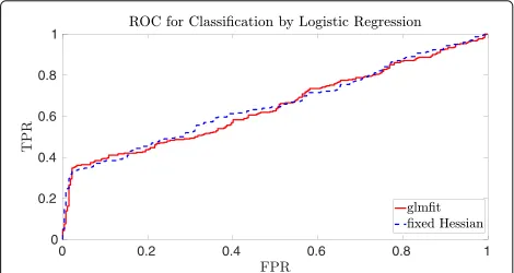
By computing the TPR and FPR for varying thresholds 0 ≤ τ ≤ 1, we can construct the receiver operating characteristic curve or ROC-curve. The ROC-curve is constructed by plotting the(FPR, TPR)pairs for each pos-sible value of the thresholdτ. In the ideal situation there would exists a point with (FPR, TPR) = (0, 1), which would imply that there exists a threshold for which the model classifies all test data correctly.
The area under the ROC-curve or AUC-value will be used as the main indicator of how well the classifier works. Since our SFH method combines several approximations, we need to verify the accuracy of our model first on unen-crypted data and later on enunen-crypted data. For well chosen system parameters, there will be no difference between accuracy for unencrypted vs. encrypted data since all computations on encrypted data are exact.
The first step is performed by comparing our SFH method with the standard logistic regression functional-ity of Matlab. This is done by applying our method with all its approximations to the plaintext data and comparing the result to the result of the “glmfit” function in Mat-lab. The functionb = glmfit(X,y, distr)returns a vector
Table 1Performance for the financial dataset with 31 covariates and 700 training records and 19,300 testing records
# iterations AUC SFH
1 0.9418
5 0.9436
10 0.9448
20 0.9466
50 0.9517
100 0.9599
Table 2Comparing actual and predicted classes
Actual class
-1 1
Predicted -1 True negative (TN) False negative (FN)
Class 1 False positive (FP) True positive (TP)
bof coefficient estimates for a generalized linear model of the responsesyon the predictors inX, using distribution distr. Generalized linear models unify various statistical models, such as linear regression, logistic regression and Poisson regression, by allowing the linear model to be related to the response variable via a link function. We use the “binomial” distribution, which corresponds to the “logit” link function andya binary vector indicating suc-cess or failure to compute the parameters of the logistic regression model with “glmfit”.
From Figs. 1 and2one can see that the SFH method classifies the data approximately as well as “glmfit” in Mat-lab, in the sense that one can always select a threshold that gives approximately the same true positive rate and false positive rate. One can thus conclude that the SFH method, with all its approximations, performs well com-pared to the standard Matlab method, which uses much more precise computations. By computing the TPR and FPR for several thresholds, we found that the approxima-tions of our SFH method shifts the model a bit such that we need a slightly larger threshold to get approximately the same TPR and FPR as for the Matlab model. Since the ideal situation would be to end up with a true posi-tive rate of 1 and false posiposi-tive rate of 0, we see from Fig.1 that for the genomics dataset both models are perform-ing rather poorly. The financial fraud use case is, however, much more amenable to binary classification as shown in Fig.2. The main conclusion is that our SFH method per-forms almost as well as standard methods such as those provided by Matlab.
0 0.2 0.4 0.6 0.8 1
0 0.2 0.4 0.6 0.8 1
Fig. 2ROC curve for the financial fraud detection with 1000 training records and 19,000 testing records, all with 31 covariates
Implementation details and performance
Our implementation uses the FV-NFLlib software library [12] which implements the FV homomorphic encryption scheme. The system parameters need to be selected taking into account the following three constraints:
1 the security of the somewhat homomorphic FV scheme,
2 the correctness of the somewhat homomorphic FV scheme,
3 the correctness of thew-NIBNAF encoding.
The security of a given set of system parameters can be estimated using the work of Albrecht, Player and Scott [13] and the open source learning with error (LWE) hard-ness estimator implemented by Albrecht [8]. This pro-gram estimates the security of the LWE problem based on the following three parameters: the degreeDof the poly-nomial ring, the ciphertext modulus q andα =
√ 2πσ
q
whereσis the standard deviation of the error distribution χerr. The security estimation is based on the best known
attacks for the learning with error problem. Our system parameters are chosen to beq = 2186,D = 4096 and σ =20 (and thusα=
√ 2πσ
q ) which results in a security of
78 bits.
As explained in the section on the FV scheme, the error in the ciphertext encrypting the result, should be small enough to enable correct decryption. By estimating the infinity norm of the noise we can select parameters that keep this noise under the correctness bound and in particular, we obtain an upper boundtmax of the
plain-text modulus. Similarly, to ensure correct decoding, the coefficients of the polynomial encoding the result must remain smaller than the size of the plaintext modulust. This condition results in a lower bound on the plaintext modulustmin.
It turns out that these bounds are incompatible for the chosen parameters, so we have to rely on the Chinese Remainder Theorem to decompose the plaintext space
into smaller parts that can be handled correctly. The plain-text modulus t is chosen as a product of small prime numberst1, t2, . . ., tnwith∀i∈ {1, . . ., n} :ti ≤tmax
andt = ni=1 ti ≥ tmin, where tmax is determined by
the correctness of the FV scheme andtminby the
correct-ness of thew-NIBNAF decoding. The CRT then gives the following ring isomorphism:
Rt→Rt1×. . .×Rtn:g(X)→(g(X)modt1, . . ., g(X)modtn). and instead of performing the training algorithm directly overRt, we compute with each of theRti’s by reducing the
w-NIBNAF encodings moduloti. The resulting choices for
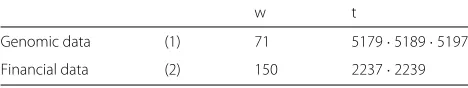
the plaintext spaces are given in Table3.
Since we are using the Chinese Remainder Theorem, each record will be encrypted using two (for the financial fraud case) or three (for the genomics case) ciphertexts. As such, a time-memory trade off is possible depending on the requirements of the application. One can choose to save computing time by executing the algorithm for the different ciphertexts in parallel; or one can choose to save memory by computing the result for each plaintext space
Rticonsecutively and overwriting the intermediate values of the computations in the process.
The memory required for each ciphertext is easy to estimate: a ciphertext consists of 2 polynomials ofRq =
Zq[X]/(XD+1), so its size is given by 2Dlog2qwhich is ≈ 186kB for the chosen parameter set. Due to the use of the CRT, we requireT (withT = 2 orT = 3) cipher-texts to encrypt each record, so the general formula for the encrypted dataset size is given by:
T(d+1)N2Dlog2q bits ,
withTthe number of prime factors used to split the plain-text modulustandd+1 (resp.N) the number of covariates (resp. records) used in the training set.
The time complexity of our SFH method is also easy to estimate, but one has to be careful to perform the operations in a specific order. If one would naively com-pute the matrixH˜ by first computingH¯ and subsequently summing each row, the complexity would be ONd2. However, the formula of thek-th diagonal element ofH˜
is given by −14 dj=1+1iN=1xk,ixj,i
, which can be
rewrit-ten as −14 Ni=1xk,i
d+1
j=1 xj,i
. This formula shows that
Table 3The parameters defining plaintext encoding
w t
Genomic data (1) 71 5179·5189·5197
Table 4Performance for the genomic dataset with a fixed number of covariates equal to 20
# training records Computation time AUC SFH AUC glmfit
500 22 min 0.6348 0.6287
600 26 min 0.6298 0.6362
800 35 min 0.6452 0.6360
1000 44 min 0.6561 0.6446
The number of testing records is for each row equal to the total number of input records (1581) minus the number of training records
it is more efficient to first sum all the rows ofXand then perform a matrix vector multiplication with complexity
O(Nd).
This complexity is clearly visible in the tables, more specifically in Tables4and5for the genomic use case, and Tables6and 7for the financial use case. All these tables show a linear growth of the computation time for a grow-ing number of records or covariates as expected by the chosen order of the computations in the implementation.
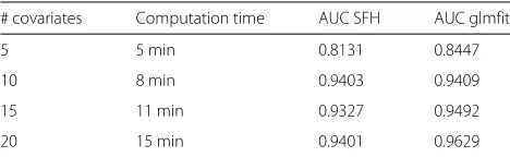
In Tables4and 5 we see that often the AUC value of the SFH model is slightly higher than the AUC value of the glmfit model. However, as mentioned before both mod-els perform poorly on this dataset. Since our SFH model contains many approximations we expect it to perform slightly worse than the “glmfit” model. Only slightly worse because Figs.1and 2already showed that the SFH mod-els classifies the data almost as well as the “glmfit” model. This is consistent with the results for the financial dataset shown in Tables6and7, which we consider more relevant than the results of the genomic dataset due to the fact that both models perform better on this dataset.
Discussion
The experiments of this article show promising results for the simple iterative method we propose as an algo-rithm to compute the logistic regression model. A first natural question is whether this technique is generaliz-able to other machine learning problems. In [14], Böhning describes how to adapt the lower bound method to make it applicable to multinomial logistic regression, it is likely this adaption will also apply to our SFH technique and hence our SFH technique can most likely also be applied to construct a multinomial logistic regression model. In
Table 5Performance for the genomic dataset with a fixed number of training records equal to 500 and the number of testing records equal to 1081
# covariates Computation time AUC SFH AUC glmfit
5 7 min 0.65 0.6324
10 12 min 0.6545 0.6131
15 17 min 0.6446 0.6241
20 22 min 0.6348 0.6272
Table 6Performance for the financial dataset with a fixed number of covariates equal to 31
# training records Computation time AUC SFH AUC glmfit
700 30 min 0.9416 0.9619
800 36 min 0.9411 0.9616
900 40 min 0.9409 0.9619
1000 45 min 0.9402 0.9668
The number of testing records is for each row equal to the total number of input records (20,000) minus the number of training records
the case of neural networks we can refer to [15]; in order to construct the neural network one needs to rank all the possibilities and only keep the best performing neurons for the next layer. Constructing this ranking homomor-phically is not straightforward and not considered at all in our algorithm, hence neural networks will require more complicated algorithms.
When we look purely at the performance of the FV homomorphic encryption scheme, we might consider a residue number system (RNS) variant of the FV scheme as described in [16] to further improve the running time of our implementation. One could also consider single instruction multiple data (SIMD) techniques as suggested in [17] or look further into a dynamic rescaling proce-dure for FV as mentioned in [6]. These techniques will presumably further decrease the running time of our implementation, which would render our solution even more valuable.
Conclusions
The simple, but effective, iterative method presented in this paper allows one to train a logistic regression model on homomorphically encrypted input data. Our method can be used to outsource the training phase of logis-tic regression to a cloud service in a privacy preserving manner. We demonstrated the performance of our logis-tic training algorithm on two real life applications using different numeric data types. In both cases, the accuracy of our method is only slightly worse than standard algo-rithms to train logistic regression models. Finally, the time complexity of our method grows linearly in the number of covariates and the number of training input data points.
Table 7Performance for the financial dataset with a fixed number of records equal to 500 and the number of testing records equal to 19,500
# covariates Computation time AUC SFH AUC glmfit
5 5 min 0.8131 0.8447
10 8 min 0.9403 0.9409
15 11 min 0.9327 0.9492
Abbreviations
AUC: Area under the curve; CRT: Chinese remainder theorem; FN: False negative; FP: False positive; FPR: False positive rate; FV: Fan vercauteren; KeyGen: Key generation; LWE: Learning with error; RNS: Residue number system; ROC: Receiver operating characteristic; SFH: Simplified fixed Hessian; SIMD: Single instruction multiple data; TN: True negative; TP: True positive; TPR: True positive rate; w-NIBNAF: w non integral base non adjacent form
Funding
This work was supported by the European Commission under the ICT programme with contract H2020-ICT-2014-1 644209 HEAT.
Availability of data and materials
The genomic dataset was available upon request during the iDASH competition. Data is still available from the authors upon request and with the permission of the organisers of the iDASH competition of 2017. The financial dataset is not publicly available. They might be made available from the authors upon request and with the permission of the specific undisclosed bank.
About this Supplement
This article has been published as part of BMC Medical Genomics Volume 11 Supplement 4, 2018: Proceedings of the 6th iDASH Privacy and Security Workshop 2017. The full contents of the supplement are available online at https://bmcmedgenomics.biomedcentral.com/articles/supplements/volume-11-supplement-4.
Authors’ contributions
Both authors worked together on the design of the solution. Both authors discussed results and wrote the manuscript together. Both authors have read and approved the manuscript.
Ethics approval and consent to participate Not applicable.
Consent for publication Not applicable.
Competing interests
The authors declare that they have no competing interests.
Publisher’s Note
Springer Nature remains neutral with regard to jurisdictional claims in published maps and institutional affiliations.
Published: 11 October 2018
References
1. Naehrig M, Lauter K, Vaikuntanathan V. Can Homomorphic Encryption Be Practical? In: Proceedings of the 3rd ACM Workshop on Cloud Computing Security Workshop, CCSW ’11. New York: ACM; 2011. p. 113–124.http://doi.acm.org/10.1145/2046660.2046682.
2. Bos JW, Lauter K, Naehrig M. Private predictive analysis on encrypted medical data. J Biomed Inform. 2014;50:234–243.
3. Aono Y, Hayashi T, Trieu Phong L, Wang L. Scalable and Secure Logistic Regression via Homomorphic Encryption. In: Proceedings of the Sixth ACM Conference on Data and Application Security and Privacy, CODASPY ’16. New York: ACM; 2016. p. 142–144.http://doi.acm.org/10.1145/ 2857705.2857731.
4. Xie W, Wang Y, Boker SM, Brown DE. PrivLogit: Efficient
Privacy-preserving Logistic Regression by Tailoring Numerical Optimizers. CoRR. 2016;abs/1611.01170.http://arxiv.org/abs/1611.01170.
5. Kim M, Song Y, Wang S, Xia Y, Jiang X. Secure logistic regression based on homomorphic encryption. IACR Cryptol ePrint Arch. 2018;2018:14. Accessed 14 Jan 2018.
6. Fan J, Vercauteren F. Somewhat practical fully homomorphic encryption. IACR Cryptol ePrint Arch. 2012;2012:144. Accessed 22 Jan 2018. 7. Lyubashevsky V, Peikert C, Regev O. On Ideal Lattices and Learning with
Errors over Rings. J ACM. 2013;60(6):43–35.https://doi.org/doi:10.1145/ 2535925.
8. Albrecht M. Complexity estimates for solving LWE. 2000.https://bitbucket. org/malb/lwe-estimator/raw/HEAD/estimator.py. Accessed 15 Aug 2017. 9. Bonte C, Bootland C, Bos JW, Castryck W, Iliashenko I, Vercauteren F.
Faster homomorphic function evaluation using non-integral base encoding. In: Fischer W, Homma N, editors. Cryptographic Hardware and Embedded Systems – CHES 2017. Cham: Springer; 2017. p. 579–600. 10. Böhning D, Lindsay BG. Monotonicity of quadratic-approximation
algorithms. Ann Inst Stat Math. 1988;40(4):641–663.
11. Gershgorin SA. Uber die abgrenzung der eigenwerte einer matrix. Bulletin de l’Académie des Sciences de l’URSS. Classe des sciences
mathématiques et na. 1931;6:749–754.
12. CryptoExperts. FV-NFLlib; 2016. https://github.com/CryptoExperts/FV-NFLlib. Accessed 10 May 2017.
13. Albrecht MR, Player R, Scott S. On the concrete hardness of learning with errors. J Math Cryptol. 2015;9(3):169–203.
14. Böhning D. Multinomial logistic regression algorithm. Ann Inst Stat Math. 1992;44(1):197–200.
15. Bos JW, Castryck W, Iliashenko I, Vercauteren F. Privacy-friendly forecasting for the smart grid using homomorphic encryption and the group method of data handling. In: Joye M, Nitaj A, editors. Progress in Cryptology - AFRICACRYPT 2017. Cham: Springer; 2017. p. 184–201. 16. Bajard J-C, Eynard J, Hasan A, Zucca V. A full rns variant of fv like
somewhat homomorphic encryption schemes. IACR Cryptol ePrint Arch. 2016;2017:22. Accessed 22 Jan 2018.