www.geosci-model-dev.net/8/1315/2015/ doi:10.5194/gmd-8-1315-2015
© Author(s) 2015. CC Attribution 3.0 License.
Structure of forecast error covariance in coupled
atmosphere–chemistry data assimilation
S. K. Park1,2,3,4, S. Lim2,3, and M. Zupanski5
1Department of Environmental Science and Engineering, Ewha Womans University, Seoul, Republic of Korea 2Department of Atmospheric Science and Engineering, Ewha Womans University, Seoul, Republic of Korea 3Center for Climate/Environment Change Prediction Research, Ewha Womans University, Seoul, Republic of Korea 4Severe Storm Research Center, Ewha Womans University, Seoul, Republic of Korea
5Cooperative Institute for Research in the Atmosphere, Colorado State University, Fort Collins, Colorado, USA
Correspondence to: S. K. Park ([email protected])
Received: 26 October 2014 – Published in Geosci. Model Dev. Discuss.: 10 December 2014 Revised: 14 April 2015 – Accepted: 16 April 2015 – Published: 5 May 2015
Abstract. In this study, we examined the structure of an ensemble-based coupled atmosphere–chemistry forecast error covariance. The Weather Research and Forecasting (WRF) model coupled with Chemistry (WRF-Chem), a cou-pled atmosphere–chemistry model, was used to create an en-semble error covariance. The control variable includes both the dynamical and chemistry model variables. A synthetic single observation experiment was designed in order to eval-uate the cross-variable components of a coupled error covari-ance. The results indicate that the coupled error covariance has important cross-variable components that allow a phys-ically meaningful adjustment of all control variables. The additional benefit of the coupled error covariance is that a cross-component impact is allowed; e.g., atmospheric obser-vations can exert an impact on chemistry analysis, and vice versa. Given the realistic structure of ensemble forecast er-ror covariance produced by the WRF-Chem, we anticipate that the ensemble-based coupled atmosphere–chemistry data assimilation will respond similarly to assimilation of real ob-servations.
1 Introduction
The regional air quality is affected by synoptic weather situ-ations or air masses with special chemical properties (Grell et al., 2000). In prediction of air quality, the coupled physical and chemical processes are essential, which include trans-port, deposition, emission, chemical transformation, aerosol
1316 S. K. Park et al.: Forecast error covariance in coupled atmosphere–chemistry data assimilation 2 Methodology and synoptic case
In this research, we use the Weather Research and Fore-casting (WRF) model coupled with Chemistry (WRF-Chem) as a prediction model (Grell et al., 2005). It simulates the emission, transport, mixing and chemical transformation of trace gases and aerosols simultaneously with meteorology and investigates the regional-scale air quality. Here, the cho-sen chemistry option is Carbon Bond Mechanism version Z (CBMZ). More details on the WRF-Chem and the cor-responding options used in this study are described in Ap-pendix A.
We chose a synoptic case on 3 September 2005 related to Typhoon Nabi (2005), characterized by an increased im-pact on the Korean Peninsula. The experiment begins at 00:00 UTC and ends at 06:00 UTC on 3 September 2005. The WRF-Chem is set up with a horizontal resolution of 30 km and 28 vertical levels. The model domain is centered over the Korean Peninsula, covering an area of approximately 3900 km×4400 km with 132×147 horizontal grid points.
The ensemble forecast includes 32 ensemble members with a 6 h assimilation window. The initial and lateral bound-ary conditions for atmospheric variables are provided by the National Center for Environmental Prediction (NCEP) Global Forecasting System (GFS), while those for chemical variables are obtained from climatology. The control vari-ables defined in DA (i.e., varivari-ables adjusted during DA) are the WRF-Chem prognostic variables that include dynamical variables such as winds, perturbation potential temperature, perturbation geopotential, water vapor mixing ratio and per-turbation dry air mass in the column, and the chemical vari-ables such as ozone (O3), nitrates (NO, NO2, NO3) and sulfur dioxide (SO2) as well.
3 Experimental design
A common approach to investigating forecast error covari-ance in data assimilation is to conduct a single observa-tion experiment (Thepaut et al., 1996; Whitaker et al., 2009; Buehner et al., 2010), in which only one observation is assim-ilated using the full DA system. The analysis increments (i.e., analysis minus guess) from such an experiment show how the observation information is distributed spatially and among different analysis variables (e.g., Buehner, 2005; Singh et al., 2011). However, in order to investigate the structure of a cou-pled forecast error covariance before real observations are available and even before the full DA algorithm is developed, one can consider the assimilation of a single synthetic obser-vation located at a chosen model grid point. In particular, we define the synthetic observation as
ysynth=xf+σo, (1)
wherexfis the forecast andσois the observation error stan-dard deviation. Following Thepaut et al. (1996, Eq. 3), with
some modifications and using Eq. (1), the analysis increment in a single synthetic observation experiment is
xa−xf=Pf σo σf2+σ2
o !
ij k
, (2)
wherexa is the analysis, σf is the forecast error standard deviation, and the subscriptij kdefines the grid location of the pseudo-observation point. Equation (2) indicates that the analysis increment represents theij kth column of the fore-cast error covariance scaled by standard deviations of obser-vation error and forecast error. In our experiments, the fore-cast error covariance is ensemble-based, as defined in Zupan-ski (2005) as
Pf= P1f/2(Pf1/2)T, P1f/2=
p1f. . . pfN,
pfn=m(x0n)−m(x0), (3)
where the superscript T denotes the transpose, the indexn refers to ensemble member,N is the total number of ensem-ble forecasts,mrepresents the nonlinear WRF-Chem model, and the subscript 0 denotes the initial time of the forecast with corresponding initial conditionsx0 and ensemble ini-tial conditionsx0n. In this experiment, the control initial con-ditions are obtained by interpolation from the NCEP GFS model, while the initial ensemble perturbations are created using the lagged forecast outputs.
Since we are interested in the coupled atmosphere– chemistry forecast error covariance, we design two experi-ments with (i) synthetic temperature observation at 250 hPa located at a grid point near (132◦E, 23◦N), on the northwest-ern side of the typhoon, and (ii) synthetic ozone observation at 250 hPa located at a grid point near the eye of the typhoon (134◦E, 21◦N).
4 Results
We show the impact of single synthetic temperature (T) and ozone (O3) observations in terms of the analysis increments xa−xfimpacting all control variables. As mentioned earlier, our main interest is to examine the cross-variable covariance structure between atmospheric and chemistry variables, since the cross-variable analysis impact is possible only because of the multivariate structure of the coupled ensemble forecast error covariance.
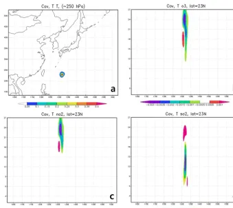
Figure 1. The analysis increments(xa−xf)in response to a singleT observation at 250 hPa (nearσ level 24): (a) horizontal response of T at 250 hPa, and vertical responses of (b) O3, (c) NO2and (d) SO2. In (b)–(d), the vertical axis represents the verticalσ levels. Units are ppmv for chemical variables and K for temperature.
change at the level of single T observation, while the SO2 analysis (Fig. 1d) is mostly impacted near 700 hPa (approx-imatelyσ level 13). This is likely a consequence of the ver-tical structure of O3and NO2, with the largest values in the upper troposphere and the stratosphere, while SO2typically has the largest values in the lower troposphere (e.g., Meena et al., 2006). The strongest impact ofT observation is on O3, with the magnitude up to 0.003 ppmv, while the magnitude is somewhat smaller for NO2and SO2. One can also infer that an increase inT will imply a decrease in O3, NO2, and SO2. Probably the most important implication of these results is that observations of an atmospheric variable (e.g., tempera-ture) can change the analysis of chemical variables in a phys-ically meaningful way. This means that, even with no chem-istry observations in the local area, the analysis of chemical variables can still be adjusted in agreement with standard dy-namical variables of the model. On the other hand, if there are chemistry observations in the area, the chemistry analy-sis change introduced by atmospheric observations will act as an additional dynamical constraint on the final analysis.
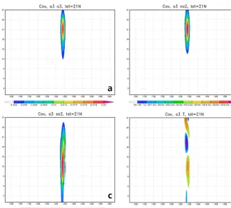
In Fig. 2, the impact of O3single observation at 250 hPa on itself and the other variables is shown. As before, we focus on the vertical cross section of the analysis response. The impact of O3observation on its own analysis shows the anticipated
response, with the largest magnitude at the observation loca-tion, approximately 0.02 ppmv (Fig. 2a). Although smaller in magnitude, the analysis increments of NO2(Fig. 2b) and SO2 (Fig. 2c) show the vertical structure with maxima in the up-per and lower troposphere, respectively. It is also notable that an increase in O3brings about an increase in NO2and SO2, confirming the direct relationship between these variables as noticed in Fig. 1. The T analysis increment indicates that there is a cooling at the level of O3observation, while there is a warming above and below (Fig. 2d).
The results shown in Figs. 1 and 2 indirectly confirm that the improved stratospheric ozone distribution by DA can make a better representation of stratospheric temperature and other constituents (e.g., Lahoz et al., 2007).
5 Conclusions
meaning-1318 S. K. Park et al.: Forecast error covariance in coupled atmosphere–chemistry data assimilation
Figure 2. Same as in Fig. 1 but for the vertical cross section of the analysis increments(xa−xf)in response to a single O3observation at 250 hPa for (a) O3, (b) NO2, (c) SO2and (d)T.
ful adjustment of all control variables, and a much wider im-pact of observations (e.g., atmospheric observation on chem-istry analysis, and vice versa). The analysis increments cre-ated in response to synthetic temperature and ozone obser-vations illustrate the complexity of atmosphere–chemistry cross-correlations and the forecast error covariance structure. Given the realistic structure of ensemble forecast error co-variance produced by the WRF-Chem, we anticipate that the ensemble-based coupled atmosphere–chemistry data
Appendix A: Description of the WRF-Chem
In this research, we use the Weather Research and Forecast-ing (WRF) model coupled with Chemistry (WRF-Chem) ver-sion 3.4.1 as a prediction model on a regional scale. As a cou-pled model, it simulates the emission, transport, mixing and chemical transformation of trace gases and aerosols simul-taneously with meteorology using the governing equations with mass and scalar conserving flux form and the terrain-following mass vertical coordinate system (Grell et al., 2005; Fast et al., 2006). Therefore, it uses the same transport scheme, horizontal and vertical coordinates, and physics schemes with the same time step (Grell et al., 2005; Fast et al., 2006). Figure A1 represents the flowchart of the WRF-Chem model. It is made up of the WRF Pre-processing System (WPS), the WRF-Chem model, and the visualiza-tion processes. The WPS creates the meteorology data with the terrestrial data and the meteorology initial conditions (ICs) and boundary conditions (BCs), which are provided by the National Center for Environmental Prediction (NCEP) Global Forecasting System (GFS) producing the global lati-tude/longitude 1 degree resolution and terrestrial data. In the WRF-Chem model, the chemical ICs and BCs are automati-cally obtained by the climatology. Furthermore, it simulates the evolution of chemical species with the prognostic vari-ables that include both dynamical and chemical varivari-ables. For the ensemble experiments, the initial ensemble pertur-bations are created using the 12 h lagged forecast outputs. Finally, the Advanced Research WRF post-processing (AR-Wpost), along with the Grid Analysis and Display System (GrADS), is used for the visualization process.
Figure A1. Flowchart of the WRF-Chem model.
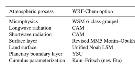
We also discuss various physical and chemical processes employed in the WRF-Chem model in more detail. Table A1 summarizes the WRF-Chem configuration options that are used in this study. To evaluate the cross-variable compo-nent of forecast error covariance, we select the simplified physical processes rather than sophisticated ones. Regard-ing the atmospheric processes, we use the recommended physics options for the regional climate case at 30 km grid size in our experiments. As the chemical options, the Carbon Bond Mechanism version Z (CBM-Z) without a dimethyl-sulfide scheme is used for the gas-phase chemistry. The CBM-Z photochemical mechanism contains 55 prognostic species and 134 reactions having the lumped structure ap-proach for condensing organic chemical species and reac-tions (Fast et al., 2006). It also uses a regime-dependent ap-proach based on the partitioned kinetics, such as background, anthropogenic, and biogenic submechanisms for saving the computational time (Fast et al., 2006). Furthermore, we con-sider the chemical tendency diagnostic for equation budget analysis. However, we did not consider the convective pa-rameterization, which can simulate the subgrid convective transport, wet scavenging, and aqueous chemistry due to a simple experiment setting, even with a typhoon case.
Table A1. Selected WRF-Chem configuration options.
Atmospheric process WRF-Chem option
Microphysics WSM 6-class graupel
Longwave radiation CAM
Shortwave radiation CAM
Surface layer Revised MM5 Monin–Obukhov
Land surface Unified Noah LSM
Planetary boundary layer YSU
Cumulus parameterization Kain–Fritsch (new Eta)
1320 S. K. Park et al.: Forecast error covariance in coupled atmosphere–chemistry data assimilation
Acknowledgements. This work is supported by the Korea En-vironmental Industry & Technology Institute through the Eco Innovation Program (ARQ201204015), and partly by the National Research Foundation of Korea Grant (no. 2009-0083527) funded by the Korean government (MSIP). The third author acknowledges partial support from National Science Foundation Collaboration in Mathematical Geosciences grant 0930265 and from NASA Model-ing, Analysis and Prediction (MAP) program grant NNX10AG92G.
Edited by: A. Sandu
References
Buehner, M.: Ensemble-derived stationary and flow-dependent background-error covariances, Q. J. R. Meteorol. Soc., 131, 1013–1043, 2005.
Buehner, M., Houtekamer, P. L., Charette, C., Mitchell, H. L., and He, B.: Intercomparison of variational data assimilation and the ensemble kalman filter for global deterministic NWP. Part I: Description and single-observation experiments, Mon. Weather Rev., 138, 1567–1586, 2010.
Constantinescu, E. M., Chai, T., Sandu, A., and Carmichael, G. R.: Autoregressive models of background errors for chemical data assimilation, J. Geophys. Res., 112, D12309, doi:10.1029/2006JD008103, 2007.
Eibern, H. and Schmidt, H.: A four-dimensional variational chem-istry data assimilation scheme for Eulerian chemchem-istry transport modeling, J. Geophys. Res., 104, 18583–18598, 1999.
Evensen, G.: The ensemble Kalman filter: theoretical formula-tion and practical implementaformula-tion, Ocean Dynam., 53, 343–367, 2003.
Fast, J. D., Gustafson Jr., W. I., Easter, R. C., Zaveri, R. A., Barnard, J. C., Chapman, E. G., Grell, G. A., and Peckham, S. E.: Evolution of ozone, particulates, and aerosol direct radia-tive forcing in the vicinity of Houston using a fully coupled meteorology-chemistry-aerosol model, J. Geophys. Res., 111, D21305, doi:10.1029/2005JD006721, 2006.
Grell, G. A., Emeis, S., Stockwell, W. R., Schoenemeyer, T., Forkel, R., Michalakes, J., Knoche, R., and Seidl, W.: Application of a multiscale, coupled MM5/chemistry model to the complex ter-rain of the VTALP valley campaign, Atmos. Environ., 34, 1435– 1453, 2000.
Grell, G. A., Peckham, S. E., Schmitz, R., McKeen, S. A., Frost, G., Skamarock, W. C., and Eder, B.: Fully coupled “online” chem-istry within the WRF model, Atmos. Environ., 39, 6957–6975, 2005.
Houtekamer, P. L. and Mitchell, H. L.: Data assimilation using an ensemble Kalman filter technique, Mon. Weather Rev., 126, 796– 811, 1998.
Lahoz, W. A., Errera, Q., Swinbank, R., and Fonteyn, D.: Data as-similation of stratospheric constituents: a review, Atmos. Chem. Phys., 7, 5745–5773, doi:10.5194/acp-7-5745-2007, 2007. Meena, G. S., Bhosale, C. S., and Jadhav, D. B.: Retrieval of
strato-spheric O3and NO2vertical profiles using zenith scattered light observations, J. Earth Syst. Sci., 115, 333–347, 2006.
Navon, I. M.: Data assimilation for numerical weather prediction: A review, in: Data Assimilation for Atmospheric, Oceanic and Hydrologic Applications, edited by: Park, S. K. and Xu, L., Springer, Berlin-Heidelberg, 21–65, 2009.
Park, S. K. and Zupanski, D.: Four-dimensional variational data as-similation for mesoscale and storm-scale applications, Meteorol. Atmos. Phys., 82, 173–208, 2003.
Singh, K., Jardak, M., Sandu, A., Bowman, K., Lee, M., and Jones, D.: Construction of non-diagonal background error covariance matrices for global chemical data assimilation, Geosci. Model Dev. Discuss., 3, 1783–1827, doi:10.5194/gmdd-3-1783-2010, 2010.
Thepaut, J.-N., Courtier, P., Belaud, G., and Lemaitre, G.: Dynami-cal structure functions in a four-dimensional variational assimila-tion: A case study, Q. J. R. Meteorol. Soc., 122, 535–561, 1996. Wang, K.-Y., Lary, D. J., Shallcross, D. E., Hall, S. M., and Pyle, J. A.: A review on the use of the adjoint method in four-dimensional atmospheric-chemistry data assimilation, Q. J. R. Meteorol. Soc., 127, 2181–2204, 2001.
Whitaker, J. S., Compo, G. P., and Thepaut, J.-N.: A comparison of variational and ensemble-based data assimilation systems for re-analysis of sparse observations, Mon. Weather Rev., 137, 1991– 1999, 2009.
Zupanski, M.: Maximum likelihood ensemble filter: Theoretical as-pects, Mon. Weather Rev., 133, 1710–1726, 2005.