www.geosci-model-dev.net/8/2515/2015/ doi:10.5194/gmd-8-2515-2015
© Author(s) 2015. CC Attribution 3.0 License.
The Parallelized Large-Eddy Simulation Model (PALM) version 4.0
for atmospheric and oceanic flows: model formulation, recent
developments, and future perspectives
B. Maronga1, M. Gryschka1, R. Heinze1, F. Hoffmann1, F. Kanani-Sühring1, M. Keck1, K. Ketelsen2, M. O. Letzel3, M. Sühring1, and S. Raasch1
1Institute of Meteorology and Climatology, Leibniz Universität Hannover, Hannover, Germany 2Software Consultant, Berlin, Germany
3Ingenieurbüro Lohmeyer GmbH & Co. KG, Karlsruhe, Germany
Correspondence to: B. Maronga ([email protected])
Received: 14 December 2014 – Published in Geosci. Model Dev. Discuss.: 19 February 2015 Revised: 6 July 2015 – Accepted: 13 July 2015 – Published: 13 August 2015
Abstract. In this paper we present the current version of the Parallelized Large-Eddy Simulation Model (PALM) whose core has been developed at the Institute of Meteorology and Climatology at Leibniz Universität Hannover (Germany). PALM is a Fortran 95-based code with some Fortran 2003 extensions and has been applied for the simulation of a va-riety of atmospheric and oceanic boundary layers for more than 15 years. PALM is optimized for use on massively parallel computer architectures and was recently ported to general-purpose graphics processing units. In the present pa-per we give a detailed description of the current version of the model and its features, such as an embedded Lagrangian cloud model and the possibility to use Cartesian topography. Moreover, we discuss recent model developments and future perspectives for LES applications.
1 Introduction
In meteorology, large-eddy simulation (LES) has been used since the early 1970s for various research topics on turbulent flows at large Reynolds numbers in the atmospheric bound-ary layer (ABL). The first investigations using LES were per-formed by Lilly (1967) and Deardorff (1973, 1974). Nowa-days, thanks to the increasing power of modern supercom-puters, the technique is well known and widely spread within the boundary-layer meteorology community (see the review in Mason, 1994). Numerous studies in boundary-layer
re-search that made use of LES have been published since then, with gradually increasing model resolution over the years (Moeng, 1984; Mason, 1989; Wyngaard et al., 1998; Sul-livan et al., 1998; Sorbjan, 2007; Maronga, 2014, among many others). A detailed intercomparison of different LES codes can be found in Beare et al. (2006). LES models solve the three-dimensional (3-D) prognostic equations for mo-mentum, temperature, humidity, and other scalar quantities. The principle of LES is based on the separation of scales. Turbulence scales that are larger than a certain filter width are directly resolved, whereas the effect of smaller scales is parametrized by a subgrid-scale (SGS) turbulence model. As the bulk part of the energy is contained in the large ed-dies, about 90 % of the turbulence energy can be resolved by means of LES (e.g., Heus et al., 2010). In practice, the filter width often depends on the grid resolution and therefore on the phenomenon that is studied. Typical filter widths can thus range from 50–100 m for phenomena on a regional scale like Arctic cold-air outbreaks (e.g., Gryschka and Raasch, 2005) down to 0.5–2 m for LES of the urban boundary layer with very narrow streets (e.g., Kanda et al., 2013), or for simula-tions of the stable boundary layer (e.g., Beare et al., 2006).
Figure 1. The PALM logo introduced in version 4.0.
later and its first formulation can be found in Raasch and Schröter (2001). Therewith, PALM was one of the first par-allelized LES models for atmospheric research at all. Many people have helped in developing the code further over the past 15 years, and large parts of the code have been added, optimized and improved since then. For example, embedded models such as a Lagrangian cloud model (LCM) as part of a Lagrangian particle model (LPM) and a canopy model have been implemented. Also, an option for Cartesian topogra-phy is available. Moreover, the original purpose of the model to study atmospheric turbulence was extended by an option for oceanic flows. Thus, Raasch and Schröter (2001) can no longer be considered an adequate reference for current and future research articles.
In the present paper we will provide a comprehensive de-scription of the current version 4.0 of PALM. The idea for this overview paper was also partly inspired by Heus et al. (2010), who gave a detailed description of the Dutch Atmo-spheric Large-Eddy Simulation (DALES) model.
In the course of the release of PALM 4.0, a logo was de-signed, showing a palm tree – a reference to the acronym PALM (see Fig. 1).
Over the last 15 years, PALM has been applied for the sim-ulation of a variety of boundary layers, ranging from hetero-geneously heated convective boundary layers (e.g., Raasch and Harbusch, 2001; Letzel and Raasch, 2003; Maronga and Raasch, 2013), urban canopy flows (e.g., Park et al., 2012; Kanda et al., 2013), and cloudy boundary layers (e.g., Riechelmann et al., 2012; Hoffmann et al., 2015; Heinze et al., 2015). Moreover, it has been used for studies of the oceanic mixed layer (OML, e.g., Noh et al., 2010, 2011) and recently for studying the feedback between atmosphere and ocean by Esau (2014). PALM also participated in the first in-tercomparison of LES models for the stable boundary layer, as part of the Global Energy and Water Cycle Experiment At-mospheric Boundary Layer Study initiative (GABLS, Beare et al., 2006). In this experiment, PALM was for the first time successfully used with extremely fine grid spacings of down to 1 m. From the very beginning, PALM was designed and optimized to run very high-resolution setups and large model domains efficiently on the world’s biggest supercomputers.
The paper is organized as follows: Sect. 2 deals with the description of the model equations, numerical methods and parallelization principles. Section 3 describes the embedded
models such as cloud physics, canopy model and LPM, fol-lowed by an overview of the technical realization (Sect. 4). In Sect. 5 we will outline topics of past applications of PALM and discuss both upcoming code developments and future perspectives of LES applications in general. Section 7 gives a summary.
2 Model formulation
In this section we will give a detailed description of the model. We will confine ourselves to the atmospheric formu-lation and devote a separate section (see Sect. 2.7) to the ocean option. By default, PALM has six prognostic quan-tities: the velocity componentsu, v, w on a Cartesian grid, the potential temperatureθ, specific humidityqv or a pas-sive scalars, and the SGS turbulent kinetic energy (SGS– TKE)e. The separation of resolved scales and SGS is im-plicitly achieved by averaging the governing equations (see Sect. 2.1) over discrete Cartesian grid volumes as proposed by Schumann (1975). Moreover, it is possible to run PALM in a direct numerical simulation mode by switching off the prognostic equation for the SGS–TKE and setting a constant eddy diffusivity. For a list of all symbols and parameters that we will introduce in Sect. 2.1, see Tables 1 and 2.
2.1 Governing equations
The model is based on the non-hydrostatic, filtered, incompressible Navier–Stokes equations in Boussinesq-approximated form. In the following set of equations, angle brackets denote a horizontal domain average. A subscript 0 indicates a surface value. Note that the variables in the equa-tions are implicitly filtered by the discretization (see above), but that the continuous form of the equations is used here for convenience. A double prime indicates SGS variables. The overbar indicating filtered quantities is omitted for readabil-ity, except for the SGS flux terms. The equations for the con-servation of mass, energy and moisture, filtered over a grid volume on a Cartesian grid, then read as
∂ui
∂t = −
∂uiuj
∂xj
−εij kfjuk+εi3jf3ug,j− 1
ρ0
∂π∗ ∂xi
(1)
+gθv− hθvi
hθvi
δi3−
∂ ∂xj
u00iu00j−2
3eδij
,
∂uj
∂xj
=0, (2)
∂θ
∂t = −
∂ujθ
∂xj
− ∂
∂xj
u00jθ00− LV
cp5
9qv, (3)
∂qv
∂t = −
∂ujqv
∂xj
− ∂
∂xj
u00jq00
v
+9qv, (4)
∂s
∂t = −
∂ujs
∂xj
− ∂
∂xj
u00js00+9
Table 1. List of general model parameters.
Symbol Value Description
cm 0.1 SGS model constant
cp 1005 J kg−1K−1 Heat capacity of dry air at constant pressure
g 9.81 m s−2 Gravitational acceleration
LV 2.5×10⁶J kg−1 Latent heat of vaporization
p0 1000 hPa Reference air pressure
Rd 287 J kg−1K−1 Specific gas constant for dry air
Rv 461.51 J kg−1K−1 Specific gas constant for water vapor
κ 0.4 Kármán constant
ρ kg m−3 Density of dry air
ρ0 1.0 kg m−3 Density of dry air at the surface
ρl,0 1003 kg m−3 Density of liquid water
0.729×10⁻⁴rad s−1 Angular velocity of the Earth
Here, i, j, k∈ {1,2,3}.ui are the velocity components (u1=u, u2=v, u3=w) with location xi (x1=x, x2=
y, x3=z), t is time, fi=(0,2cos(φ),2sin(φ)) is the Coriolis parameter with being the Earth’s angular ve-locity and φ being the geographical latitude. ug,k are the geostrophic wind speed components,ρ0is the density of dry air, π∗=p∗+2
3ρ0e is the modified perturbation pressure withp∗being the perturbation pressure and the SGS–TKE
e=1
2u
00
iu
00
i, and gis the gravitational acceleration. The po-tential temperature is defined as
θ=T / 5, (6)
with the current absolute temperatureT and the Exner func-tion
5=
p
p0 Rd/cp
, (7)
with p being the hydrostatic air pressure, p0=1000 hPa a reference pressure,Rdthe specific gas constant for dry air, andcp the specific heat of dry air at constant pressure. The virtual potential temperature is defined as
θv=θ
1+ R
v
Rd
−1
qv−ql
, (8)
with the specific gas constant for water vaporRv, and the liq-uid water specific humidityql. For the computation ofql, see the descriptions of the embedded cloud microphysical mod-els in Sects. 3.1 and 3.3. Furthermore,LV is the latent heat of vaporization, and9qv and9s are source/sink terms ofqv ands, respectively.
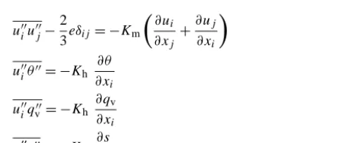
2.2 Turbulence closure
One of the main challenges in LES modeling is the turbu-lence closure. The filtering process yields four SGS covari-ance terms (see Eqs. 1–5) that cannot be explicitly calculated.
In PALM, these SGS terms are parametrized using a 1.5-order closure after Deardorff (1980). PALM uses the mod-ified version of Moeng and Wyngaard (1988) and Saiki et al. (2000). The closure is based on the assumption that the en-ergy transport by SGS eddies is proportional to the local gra-dients of the mean quantities and reads
u00iu00j−2
3eδij= −Km ∂u
i
∂xj
+∂uj
∂xi
(9)
u00iθ00= −K
h
∂θ ∂xi
(10)
u00iq00
v = −Kh
∂qv
∂xi
(11)
u00is00= −K
h
∂s ∂xi
, (12)
whereKmandKhare the local SGS eddy diffusivities of mo-mentum and heat, respectively. They are related to the SGS– TKE as follows:
Km=cml
√
e, (13)
Kh=
1+2l
1
Km. (14)
Here,cm=0.1 is a model constant and1= 3
√
1x1y1z
with1x,1y,1zbeing the grid spacings in thex,y andz
directions, respectively. The SGS mixing lengthldepends on heightz(distance from the wall when topography is used), 1, and stratification, and is calculated as
l=
min
1.8z,1,0.76√e
g θv,0
∂θv ∂z
−12 for∂θv
∂z >0,
min(1.8z,1) for∂θv
∂z ≤0. (15)
Moreover, the closure includes a prognostic equation for the SGS–TKE:
∂e ∂t = −uj
∂e ∂xj
−u00iu00j∂ui ∂xj
+ g
θv,0
Table 2. List of general symbols.
Symbol Dimension Description
Crelax m−1 Relaxation coefficient for laminar inflow
D m Length of relaxation area for laminar inflow
d m Distance to the inlet
e m2s−2 SGS–TKE
Finflow m−1 Damping factor for laminar inflow
f s−1 Coriolis parameter
Kh m2s−1 SGS eddy diffusivity of heat
Km m2s−1 SGS eddy diffusivity of momentum
L m Obukhov length
l m SGS mixing length
lBl m Mixing length in the free atmosphere after Blackadar (1997)
p hPa Hydrostatic pressure
p∗ hPa Perturbation pressure
Qθ K m s−1 Upward vertical kinematic heat flux
q kg kg−1 Total water content
ql kg kg−1 Liquid water specific humidity
qv kg kg−1 Specific humidity
q∗ kg kg−1 MOST humidity scale
Ri Gradient Richardson number
s kg m−3 Passive scalar
Uui m s
−1 Transport velocity of the indexed velocity component at the outlet
ug,i m s−1 Geostrophic wind components (ug,1=ug, ug,2=vg)
ui m s−1 Velocity components (u1=u, u2=v, u3=w)
ui,LS m s−1 Large-scale advection velocity components
u∗ m s−1 Friction velocity
xi m Coordinate on the Cartesian grid (x1=x, x2=y, x3=z)
xinlet m Position of the inlet
xrecycle m Distance of the recycling plane from the inlet
z0 m Roughness length for momentum
z0,h m Roughness length for heat
zMO m Height of the constant flux layer (MOST)
α Angle between thexdirection and the wind direction
1 m Nominal grid spacing
1 Difference operator
1x, 1y, 1z m Grid spacings inx, y, zdirection
1t s Time step of the LES model
δ Kronecker delta
ε Levi-Civita symbol
m2s−3 SGS–TKE dissipation rate
θ K Potential temperature
θinflow K Laminar inflow profile ofθ
θl K Liquid water potential temperature
θv K Virtual potential temperature
θ∗ K MOST temperature scale
5 Exner function
τLS s Relaxation timescale for nudging
8h Similarity function for heat
8m Similarity function for momentum
ϕ A prognostic variable (u, v, w, θ/θl, qv/q, s, e)
ϕLS Large-scale value ofϕ
9qv kg kg
−1s−1 Source/sink term ofq v
− ∂
∂xj "
u00j
e+p
00
ρ0 #
−. (16)
The pressure term in Eq. (16) is parametrized as "
u00j
e+p
00
ρ0 #
= −2Km
∂e ∂xj
(17)
andis the SGS dissipation rate within a grid volume, given by
=
0.19+0.74l 1
e32
l . (18)
Sinceθvdepends onθ,qv, andql(see Eq. 8), the vertical SGS buoyancy flux w00θ
v00 depends on the respective SGS fluxes (Stull, 1988, Chap. 4.4.5):
w00θ
v00=K1·w00θ00+K2·w00qv00−θ·w00ql00, (19) with
K1=1+
R v
Rd
−1
qv−ql, (20)
K2=
R v
Rd
−1
θ, (21)
and the vertical SGS flux of liquid water, calculated as
w00q
l00= −Kh
∂ql
∂z. (22)
Note that this parametrization of the SGS buoyancy flux (Eq. 19) differs from that used with bulk cloud microphysics (see Sect. 3.1.8).
2.3 Discretization
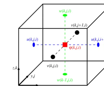
The model domain in PALM is discretized in space using fi-nite differences and equidistant horizontal grid spacings (1x,
1y). The grid can be stretched in the vertical direction well above the ABL to save computational time in the free atmo-sphere. The Arakawa staggered C-grid (Harlow and Welch, 1965; Arakawa and Lamb, 1977) is used, where scalar quan-tities are defined at the center of each grid volume, whereas velocity components are shifted by half a grid width in their respective direction so that they are defined at the edges of the grid volumes (see Fig. 2). It is thus possible to calculate the derivatives of the velocity components at the center of the volumes (same location as the scalars). By the same to-ken, derivatives of scalar quantities can be calculated at the edges of the volumes. In this way it is possible to calculate derivatives over only one grid length and the effective spatial model resolution can be increased by a factor of 2 in compar-ison to non-staggered grids.
By default, the advection terms in Eqs. (1)–(5) are dis-cretized using an upwind-biased fifth-order differencing
x,i y,j z,k
ϕ(k,j,i)
u(k,j,i+1) u(k,j,i)
w(k,j,i)
w(k-1,j,i)
v(k,j+1,i)
v(k,j,i)
Figure 2. The Arakawa staggered C-grid. The indicesi,j andk
refer to grid points in thex,yandzdirections, respectively. Scalar quantitiesϕare defined at the center of the grid volume, whereas velocities are defined at the edges of the grid volumes.
scheme in combination with a third-order Runge–Kutta time-stepping scheme after Williamson (1980). Wicker and Ska-marock (2002) compared different time and advection dif-ferencing schemes and found that this combination gives the best results regarding accuracy and algorithmic simplic-ity. However, the fifth-order differencing scheme is known to be overly dissipative. It is thus also possible to use a second-order scheme after Piacsek and Williams (1970). The latter scheme is non-dissipative, but it suffers from im-mense numerical dispersion. Time discretization can also be achieved using second-order Runge–Kutta or first-order Eu-ler schemes.
2.4 Pressure solver
The Boussinesq approximation requires incompressibility of the flow, but the integration of the governing equations for-mulated in Sect. 2.1 does not provide this feature. Diver-gence of the flow field is thus inherently produced. Hence, a predictor–corrector method is used where an equation is solved for the modified perturbation pressure after every time step (e.g., Patrinos and Kistler, 1977). In a first step, the pres-sure term−(1/ρ0)∂π∗/∂xi is excluded from Eq. (1) during time integration. This yields a preliminary velocityuti,pre+1t at timet+1t. Emerging divergences can then be attributed to the pressure term. Subsequently, the prognostic velocity can be decomposed in a second step as
uti+1t=uti,pre+1t−1t· 1
ρ0
∂π∗t ∂xi
. (23)
The third step then is to stipulate incompressibility for
uti+1t:
∂ ∂xi
uti+1t= ∂
∂xi
uti,pre+1t−1t· 1
ρ0
∂π∗t ∂xi
!
The result is a Poisson equation forπ∗:
∂2π∗t ∂xi2 =
ρ0
1t ∂uti,pre+1t
∂xi
. (25)
The exact solution of Eq. (25) would give aπ∗that yields auti+1t free of divergence when used in Eq. (23). In prac-tice, a numerically efficient reduction of divergence by sev-eral orders of magnitude is found to be sufficient. Note that the differentials in Eqs. (23)–(25) are used for convenience and that the model code uses finite differences instead. When employing a Runge–Kutta time stepping scheme, the formu-lation above is used to solve the Poisson equation for each substep.π∗is then calculated from its weighted average over these substeps.
In the case of cyclic lateral boundary conditions, the solution of Eq. (25) is achieved by using a direct fast Fourier transform (FFT). The Poisson equation is Fourier transformed in both horizontal directions; the resulting tri-diagonal matrix is solved along the z direction, and then transformed back (see, e.g., Schumann and Sweet, 1988). PALM provides the inefficient but less restrictive Singleton FFT (Singleton, 1969) and the well-optimized Temperton FFT (Temperton, 1992). External FFT libraries can be used as well, with the FFTW (Frigo and Johnson, 1998) being the most efficient one. Alternatively, the iterative multigrid scheme can be used (e.g., Hackbusch, 1985). This scheme uses an iterative successive over-relaxation (SOR) method for the inner iterations on each grid level. The convergence of this scheme is steered by the number of so-called V- or W-cycles to be carried out for each call of the scheme and by the number of SOR iterations to be carried out on each grid level. As the multigrid scheme does not require periodicity along the horizontal directions, it allows for using non-cyclic lateral boundary conditions.
2.5 Boundary conditions
PALM offers a variety of boundary conditions. Dirichlet or Neumann boundary conditions can be chosen foru,v,θ,qv, and p∗ at the bottom and top of the model. For the hori-zontal velocity components the choice of Neumann (Dirich-let) boundary conditions yields free-slip (no-slip) conditions. Neumann boundary conditions are also used for the SGS– TKE. Kinematic fluxes of heat and moisture can be pre-scribed at the surface instead (Neumann conditions) of tem-perature and humidity (Dirichlet conditions). At the top of the model, Dirichlet boundary conditions can be used with given values of the geostrophic wind. By default, the lowest grid level (k=0) for the scalar quantities and horizontal ve-locity components is not staggered vertically and defined at the surface (z=0). In case of free-slip boundary conditions at the bottom of the model, the lowest grid level is defined be-low the surface (z= −0.5·1z) instead. Vertical velocity is assumed to be zero at the surface and top boundaries, which implies using Neumann conditions for pressure.
Following Monin–Obukhov similarity theory (MOST), a constant flux layer can be assumed as the boundary condi-tion between the surface and the first grid level where scalars and horizontal velocities are defined (k=1,zMO=0.5·1z). It is then required to provide the roughness lengths for mo-mentumz0and heatz0,h. Momentum and heat fluxes as well as the horizontal velocity components are calculated using the following framework. The formulation is theoretically only valid for horizontally averaged quantities. In PALM we assume that MOST can also be applied locally and we there-fore calculate local fluxes, velocities, and scaling parameters. Following MOST, the vertical profile of the horizontal wind velocityuh=(u2+v2)
1
2 is given in the surface layer by
∂uh
∂z =
u∗
κz8m
z
L
, (26)
whereκ=0.4 is the Von Kármán constant and 8m is the similarity function for momentum in the formulation of Businger–Dyer (see, e.g., Panofsky and Dutton, 1984):
8m=
(
1+5Lz for Lz ≥0 1−16Lz−
1 4 for z
L<0.
(27)
Here,Lis the Obukhov length, calculated as
L= θv(z)u
2
∗
κgθ∗+0.61θ (z)q∗+0.61qv(z)θ∗
. (28)
The scaling parametersθ∗andq∗are defined by MOST as
θ∗= −
w00θ00
0
u∗
, q∗= −
w00q00
v 0
u∗
, (29)
with the friction velocityu∗defined as
u∗=
u00w00
0 2
+v00w00
0 2
1 4
. (30)
In PALM,u∗is calculated fromuhatzMOby vertical in-tegration of Eq. (26) overzfromz0tozMO.
From Eqs. (26) and (30) it is possible to derive a formula-tion for the horizontal wind components, viz.
∂u
∂z =
−u00w00
0 u∗κz
8m z L and ∂v ∂z =
−v00w00
0 u∗κz
8m
z
L
. (31)
Vertical integration of Eq. (31) overzfromz0tozMOthen yields the surface momentum fluxesu00w00
0andv00w000. The formulations above all require knowledge of the scal-ing parametersθ∗ andq∗. These are deduced from vertical
integration of
∂θ
∂z =
θ∗
κz8h
z
L
and∂qv
∂z =
q∗
κz8h
z
L
overzfromz0,htozMO. The similarity function8his given by
8h=
(
1+5Lz forLz ≥0 1−16Lz−12
forLz <0 .
(33)
Note that this implementation of MOST in PALM requires the use of data from the previous time step. The following steps are thus carried out in sequential order. First of all,θ∗
and q∗ are calculated by integration of Eq. (32) using the
value ofzMO/Lfrom the previous time step. Second, the new value ofzMO/Lis derived from Eq. (28) using the new val-ues ofθ∗andq∗, but usingu∗from the previous time step.
Then, the new values ofu∗, and subsequentlyu00w000as well asv00w00
0, are calculated by integration of Eqs. (26) and (31), respectively. At last, Eq. (29) is employed to calculate the new surface fluxes w00θ00
0 andw00qv 000 . In the special case, when surface fluxes are prescribed instead of surface tem-perature and humidity, the first and last steps are omitted and
θ∗andq∗are directly calculated using Eq. (29) instead.
Furthermore, the flat bottom of the model can be replaced by a Cartesian topography (see Sect. 2.5.4).
By default, lateral boundary conditions are set to be cyclic in both directions. Alternatively, it is possible to opt for non-cyclic conditions in one direction, i.e., a laminar or turbu-lent inflow boundary (see Sect. 2.5.1) and an open outflow boundary on the opposite side (see Sect. 2.5.3). The bound-ary conditions for the other direction have to remain cyclic.
In order to prevent gravity waves from being reflected at the top boundary, a sponge layer (Rayleigh damping) can be applied to all prognostic variables in the upper part of the model domain (Klemp and Lilly, 1978). Such a sponge layer should be applied only within the free atmosphere, where no turbulence is present.
The model is initialized by horizontally homogeneous ver-tical profiles of potential temperature, specific humidity (or a passive scalar), and the horizontal wind velocities. The latter can also be provided from a 1-D precursor run (see Sect. 3.5). Uniformly distributed random perturbations with a user-defined amplitude can be imposed to the fields of the horizontal velocity components to initiate turbulence. 2.5.1 Laminar and turbulent inflow boundary
conditions
In case of laminar inflow, Dirichlet boundary conditions are used for all quantities, except for the SGS–TKEeand pertur-bation pressureπ∗, for which Neumann boundary conditions are used. Vertical profiles, as taken for the initialization of the simulation, are used for the Dirichlet boundary conditions. In order to allow for a fast turbulence development, random perturbations can be imposed on the velocity fields within a certain area behind the inflow boundary (inlet). These per-turbations may persist for the entire simulation. For the pur-pose of preventing gravity waves from being reflected at the
Figure 3. Schematic figure of the turbulence recycling method used for generation of turbulent inflow. The configuration represents ex-emplary conditions with a built-up analysis area (brown surface) and an open water recycling area (blue surface). The blue arrow indicates the flow direction.
inlet, a relaxation area can be defined after Davies (1976). So far, it was found to be sufficient to implement this method for temperature only. This is hence realized by an additional term in the prognostic equation forθ(see Eq. 3):
∂θ
∂t =. . .−Crelax(θ−θinlet) . (34)
Here,θinletis the stationary inflow profile ofθ, andCrelax is a relaxation coefficient, depending on the distanced from the inlet, viz.
Crelax(d)= (
Finlet·sin2 π2DD−d
ford < D,
0 ford≥D, (35)
withDbeing the length of the relaxation region and Finlet being a damping factor.
2.5.2 Turbulence recycling
If non-cyclic horizontal boundary conditions are used, PALM offers the possibility of generating time-dependent turbulent inflow data by using a turbulence recycling method. The method follows the one described by Lund et al. (1998), with the modifications introduced by Kataoka and Mizuno (2002). Figure 3 gives an overview of the recycling method used in PALM. The turbulent signalϕ0(y, z, t )is taken from a recycling plane that is located at a fixed distancexrecycle from the inlet:
ϕ0(y, z, t )=ϕ(xrecycle, y, z, t )− hϕiy(z, t ), (36) where hϕiy(z, t ) is the line average of a prognostic vari-ableϕ∈ {u, v, w, θ, e}alongyatx=xrecycle.ϕ0(y, z)is then added to the mean inflow profilehϕinflowiy(z)atxinlet after each time step:
boundary-layer depth.hϕinletiy(z)is constant in time and ei-ther calculated from the results of the precursor run or pre-scribed by the user. The distancexrecyclehas to be chosen to be much larger than the integral length scale of the respec-tive turbulent flow. Otherwise, the same turbulent structures could be recycled repeatedly, so that the turbulence spectrum is illegally modified. It is thus recommended to use a precur-sor run for generating the initial turbulence field of the main run. The precursor run can have a comparatively small do-main along the horizontal directions. In that case the dodo-main of the main run is filled by cyclic repetition of the precur-sor run data. Note that the turbulence recycling has not been adapted for humidity and passive scalars so far.
Turbulence recycling is frequently used for simulations with urban topography. In such a case, topography elements should be placed sufficiently downstream ofxrecycleto pre-vent effects on the turbulence at the inlet.
2.5.3 Open outflow boundary conditions
At the outflow boundary (outlet), the velocity componentsui meet radiation boundary conditions, viz.
∂ui
∂t +Uui ∂ui
∂n =0, (38)
as proposed by Orlanski (1976). Here∂/∂nis the derivative normal to the outlet (i.e., ∂/∂x in Fig. 3) andUui a
trans-port velocity that includes wave propagation and advection. Rewriting Eq. (38) yields the transport velocity
Uui= −
∂u i
∂t ∂ui
∂n
−1
(39)
that is calculated at interior grid points next to the outlet at the preceding time step for each velocity component. If the transport velocity, calculated by means of Eq. (39), is outside the range 0≤Uui≤1/1t, it is set to the respective
thresh-old value that is exceeded. Because this local determination ofUui can show high variations in case of complex turbulent
flows, it is averaged laterally to the direction of the outflow, so that it varies only in the vertical direction. Alternatively, the transport velocity can be set to the upper threshold value (Uui=1/1t) for the entire outlet. Equations (38) and (39)
are discretized using an upstream method following Miller and Thorpe (1981). As the radiation boundary condition does not ensure conservation of mass, a mass flux correction can be applied at the outlet.
2.5.4 Topography
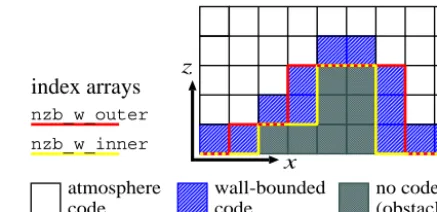
The Cartesian topography in PALM is generally based on the mask method (Briscolini and Santangelo, 1989) and allows for explicitly resolving solid obstacles such as buildings and orography. The implementation makes use of the following simplifications:
atmosphere code
z
x
index arrays
wall-bounded code
no code (obstacle) nzb_w_outer
nzb_w_inner
Figure 4. Sketch of the 2.5-D implementation of topography using the mask method (here forw). The yellow and red lines represent the limits of the arraysnzb_w_innerandnzb_w_outeras de-scribed in Sect. 4.3, respectively.
1. the obstacle shape is approximated by (an appropriate number of) full grid cells to fit the grid, i.e., a grid cell is either 100 % fluid or 100 % obstacle,
2. so far, only bottom surface-mounted obstacles are per-mitted (no holes or overhanging structures), and 3. the obstacles are fixed (not moving).
These simplifications transform the 3-D obstacle dimen-sion into a 2.5-D topography. This reduced dimendimen-sion for-mat conforms to the digital elevation model (DEM) forfor-mat. DEMs of city morphologies have become increasingly avail-able worldwide due to advances in remote sensing technolo-gies. Consequently, it is sufficient to provide 2-D topography height data to mask obstacles and their faces in PALM. The model domain is then separated into three subdomains (see Fig. 4):
A. grid points in free fluid without adjacent walls, where the standard PALM code is executed,
B. grid points next to walls that require extra code (e.g., wall functions), and
C. grid points within obstacles that are excluded from cal-culations.
Additional topography code is only executed in grid vol-umes of subdomain B. The faces of the obstacles are always located where the respective wall-normal velocity compo-nentsu,v, andware defined (cf. Fig. 2) so that the imper-meability boundary condition can be implemented by setting the respective wall-normal velocity component to zero.
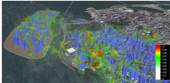
Wall surfaces in PALM can be aligned horizontally (bot-tom surface or rooftop, i.e., always facing upwards) or verti-cally (facing the north, east, south or west direction). At hor-izontal surfaces, PALM allows us to either specify the sur-face values (θ,qv,s) or to prescribe their respective surface fluxes. The latter is the only option for vertically oriented surfaces. Simulations with topography require the applica-tion of MOST between each wall surface and the first com-putational grid point. For vertical walls, neutral stratification is assumed for MOST. The topography implementation has been validated by Letzel et al. (2008) and Kanda et al. (2013). Park and Baik (2013) have recently extended the vertical wall boundary conditions for non-neutral stratifications and vali-dated their results against wind tunnel data. Up to now, how-ever, these modifications have not been included in PALM 4.0. Figure 5 shows exemplarily the development of turbu-lence structures induced by a densely built-up artificial island off the coast of Macau, China (see also animation in Knoop et al., 2014). The approaching flow above the sea exhibits relatively weak turbulence due to the smooth water surface. Within the building areas, strong turbulence is generated by additional wind shear (due to the walls of isolated buildings) and due to a general increase in surface roughness.
The technical realization of the topography will be out-lined in Sect. 4.3.
2.6 Large-scale forcing
Processes occurring on larger scales (LS) than usually con-sidered in LES and that affect the local LES scales have to be prescribed by additional source terms. These LS pro-cesses include pressure gradients via the geostrophic wind, subsidence and horizontal advection of scalars. In case of cyclic boundary conditions, this forcing is prescribed homo-geneously in the horizontal directions and thus depends on height and time only. The relation between LS pressure (pLS) gradient and geostrophic wind is given by
∂pLS
∂xi
= −ρ0εi3jf3ug,j, (40)
and enters Eq. (1). LS vertical advection (subsidence or as-cent) tendencies can be prescribed for the scalar prognostic variablesϕ∈ {θ, q, s}by means of
∂ϕ ∂t
SUB
= −wLS
∂ϕ
∂z. (41)
The so-called subsidence velocitywLSand the geostrophic wind components ug and vg can either be prescribed gradient-wise or they can be provided in an external file. Moreover, an external pressure gradient can be applied for simulations with Coriolis force switched off, which is usu-ally required for simulations to be compared with wind tun-nel experiments.
To account for less idealized flow situations, time-dependent surface fluxes (or surface temperature and humid-ity) can be prescribed. Moreover, LS horizontal advective
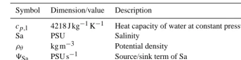
Table 3. List of ocean model parameters. Symbol Dimension/value Description
cp,l 4218 J kg−1K−1 Heat capacity of water at constant pressure
Sa PSU Salinity
ρθ kg m−3 Potential density 9Sa PSU s−1 Source/sink term of Sa
(LSA) tendencies can be added to the scalar quantities by means of
∂ϕ ∂t
LSA
= −
uLS
∂ϕLS
∂x +vLS
∂ϕLS
∂y
. (42)
These tendencies are typically derived from larger-scale models or observations and should be spatially averaged over a large domain so that local-scale perturbations are avoided.
Newtonian relaxation (nudging) towards given large-scale profilesϕLScan be used forϕ∈ {u, v, θ, q, s}via
∂ϕ ∂t
NUD
= −hϕi −ϕLS
τLS
. (43)
τLSis a relaxation timescale that, on the one hand, should be chosen large enough on the order of several hours to allow an undisturbed development of the small-scale turbulence in the LES model. On the other hand, it should be chosen small enough to account for synoptic disturbances (Neggers et al., 2012). In this way, the nudging can prevent consider-able model drift in time.
2.7 Ocean option
PALM allows for studying the OML by using an ocean op-tion where the sea surface is defined at the top of the model, so that negative values of z indicate the depth. Hereafter, we keep the terminology and use the word surface and in-dex 0 for variables at the sea surface and top of the ocean model. For a list of ocean-specific parameters, see Table 3. The ocean version differs from the atmospheric version by a few modifications, which are handled in the code by dis-tinction of cases, so that both versions share the same ba-sic code. In particular, seawater buoyancy and static stability depend not only onθ, but also on the salinity Sa. In order to account for the effect of salinity on density, a prognostic equation is added for Sa (in PSU, practical salinity unit):
∂Sa
∂t = −
∂ujSa
∂xj
− ∂
∂xj
u00jSa00+9Sa, (44)
where9Sa represents sources and sinks of salinity. Further-more,θvis replaced by potential densityρθ in the buoyancy term of Eq. (1)
+gθv− hθvi
hθvi
δi3 → −g
ρθ− hρθi
hρθi
Figure 5. Snapshot of the absolute value of the 3-D rotation vector of the velocity field (red to white colors) for a simulation of the city of Macau, including a newly built-up artificial island (left). Buildings are displayed in blue. A neutrally stratified flow was simulated with the mean flow direction from the upper left to the bottom right, i.e., coming from the open sea and flowing from the artificial island to the city of Macau. The figure shows only a subregion of the simulation domain that spanned a horizontal model domain of about 6.1×2.0×1 km3, and with an equidistant grid spacing of 8 m. The copyright for the underlying satellite image is held by Cnes/Spot Image, Digitalglobe. For more details, see the associated animation (Knoop et al., 2014).
in the stability-related term of the SGS–TKE equation (Eq. 16)
+ g
θv,0
u003θv00 → +
g ρθ,0
u003ρθ00 (46)
as well as in the calculation of the mixing length (Eq. 15) g
θv,0
∂θv
∂z
−12 →
g
ρθ,0
∂ρθ
∂z
−12
. (47)
ρθis calculated from the equation of state of seawater after each time step using the algorithm proposed by Jackett et al. (2006). The algorithm is based on polynomials depending on Sa,θ, andp (see Jackett et al., 2006, Table A2). At the moment, only the initial values ofpenter this equation.
The ocean is driven by prescribed fluxes of momentum, heat and salinity at the top. The boundary conditions at the bottom of the model can be chosen as for atmospheric runs, including the possibility to use topography at the sea bottom. Note that the current version of the ocean option does not account for the effect of surface waves (e.g., Langmuir circu-lation and wave-breaking). Parametrization schemes might, however, be provided within the user interface (see Sect. 4.5) and have been used, e.g., by Noh et al. (2004). The ocean option in its current state was recently used for simulations of the ocean mixed layer by Esau (2014), who investigated indirect air–sea interactions by means of the atmosphere– ocean coupling scheme that will be described in Sect. 2.8. Note that most previous PALM studies of the OML used the atmospheric code, subsequent inversion of thezaxis and ap-propriate normalization of the results, instead of using the relatively new ocean option (e.g., Noh et al., 2004, 2009).
2.8 Coupled atmosphere–ocean simulations
A coupled mode for the atmospheric and oceanic versions of PALM has been developed in order to allow for studying the interaction between turbulent processes in the ABL and OML. The coupling is realized by the online exchange of in-formation at the sea surface (boundary conditions) between two PALM runs (one atmosphere and one ocean). The at-mospheric model uses a constant flux layer and transfers the kinematic surface fluxes of heat and moisture as well as the momentum fluxes to the oceanic model. Flux conservation between the ocean and the atmosphere requires an adjust-ment of the fluxes for the density of waterρl,0:
w00u00
0|ocean=
ρ0
ρl,0
w00u00
0,
w00v00
0|ocean=
ρ0
ρl,0
w00v00
0. (48)
Since evaporation leads to cooling of the surface water, the kinematic flux of heat in the ocean depends on both the atmospheric kinematic surface fluxes of heat and moisture and is calculated by
w00θ00
0|ocean=
ρ0
ρl,0
cp
cp,l
w00θ00
0+
LV
cp
w00q00
0
. (49)
Here,cp,lis the specific heat of water at constant pressure. Since salt does not evaporate, evaporation of water also leads to an increase in salinity in the ocean subsurface. This pro-cess is modeled after Steinhorn (1991) by a negative (down-ward) salinity flux at the sea surface:
w00S00
0|ocean= −
ρ0
ρl,0
S
1000 PSU−Sw
00q00
Sea surface values of potential temperature and the hori-zontal velocity components are transferred as surface bound-ary conditions to the atmosphere:
θ0=θ0|ocean, u0=u0|ocean, v0=v0|ocean. (51) The time steps for atmosphere and ocean are set individ-ually and are not required to be equal. The coupling is then executed at a user-prescribed frequency. At the moment, the coupling requires equal extents of the horizontal model do-mains in both atmosphere and ocean. In order to account for the fact that eddies in the ocean are generally smaller but usually have lower velocities than in the atmosphere, it is beneficial to use different grid spacings in both models (i.e., finer grid spacing in the ocean model). In this case, the cou-pling is realized by a two-way bi-linear interpolation of the data fields at the sea surface. Furthermore, it is possible to perform uncoupled precursor runs for both atmosphere and ocean, followed by a coupled restart run. In this way it is possible to reduce the computational load due to different spin-up times in atmosphere and ocean.
As mentioned above, this coupling has been success-fully applied for the first time in the recent study of Esau (2014). Furthermore, we would encourage the atmospheric and oceanic scientific community to consider the coupled atmosphere–ocean LES technique for further applications in the future.
3 Embedded models
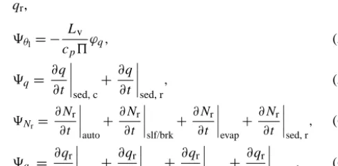
PALM offers several optional embedded models that can be switched on for special purposes. In this section we will de-scribe the embedded cloud microphysics model (Sect. 3.1, Table 4), the LPM for use of Lagrangian particles as pas-sive tracers (Sect. 3.2, Table 5), the LCM that uses the LPM for the simulation of explicit cloud droplets and aerosols (Sect. 3.3), and the canopy model (Sect. 3.4, Table 6). More-over, we will outline the one-dimensional (1-D) version of PALM in Sect. 3.5, which is used for creating steady-state wind profiles to be used as initialization of the 3-D model. 3.1 Cloud microphysics
PALM offers an embedded bulk cloud microphysics repre-sentation that takes into account the liquid water specific humidity and warm (i.e., no ice) cloud-microphysical pro-cesses. Therefore, PALM solves the prognostic equations for the total water content
q=qv+ql, (52)
instead of qv, and for a linear approximation of the liquid water potential temperature (e.g., Emanuel, 1994)
θl=θ−
LV
cp5
ql, (53)
instead of θ as described in Sect. 2.1. Since q andθl are conserved quantities for wet adiabatic processes, condensa-tion/evaporation is not considered for these variables.
Liquid-phase microphysics are parametrized following the two-moment scheme of Seifert and Beheng (2001, 2006), which is based on the separation of the droplet spectrum into droplets with radii<40 µm (cloud droplets) and droplets with radii≥40 µm (rain droplets). The model predicts the first two moments of these partial droplet spectra, namely cloud and rain droplet number concentration (NcandNr, re-spectively) as well as cloud- and rainwater specific humidity (qcandqr, respectively). Consequently,qlis the sum of both
qc andqr. The moments’ corresponding microphysical ten-dencies are derived by assuming the partial droplet spectra to follow a gamma distribution that can be described by the pre-dicted quantities and empirical relationships for the distribu-tion’s slope and shape parameters. For a detailed derivation of these terms, see Seifert and Beheng (2001, 2006).
We employ the computational efficient implementation of this scheme as used in the UCLA-LES (Savic-Jovcic and Stevens, 2008) and DALES (Heus et al., 2010) models. We thus solve only two additional prognostic equations forNr andqr:
∂Nr
∂t = −uj ∂Nr
∂xj
− ∂
∂xj
u00jN00
r
+9Nr, (54)
∂qr
∂t = −uj ∂qr
∂xj
− ∂
∂xj
u00jq00
r
+9qr, (55)
with the sink/source terms9Nrand9qr, and the SGS fluxes
u00jN00
r = −Kh
∂qr
∂xi
, (56)
u00jq00
r = −Kh
∂Nr
∂xi
(57)
Nc and qc then are a fixed parameter and a diagnostic quantity, respectively.
In the next subsections we will describe the diagnostic de-termination ofqc. From Sect. 3.1.2 on, the microphysical processes considered in the sink/source terms ofθl,q,Nrand
qr,
9θl= −
Lv
cp5
ϕq, (58)
9q=
∂q ∂t sed, c +∂q ∂t sed, r , (59)
9Nr=
∂Nr ∂t auto + ∂Nr
∂t slf/brk + ∂Nr
∂t evap + ∂Nr
∂t sed, r , (60)
9qr=
∂qr ∂t auto
+∂qr
∂t accr
+ ∂qr
∂t evap
+ ∂qr
∂t sed, r , (61)
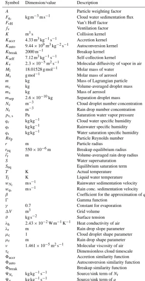
Table 4. List of cloud physics parameters and symbols.
Symbol Dimension/value Description
A Particle weighting factor
Fqc kg m
−3m s−1 Cloud water sedimentation flux
FvH Van’t Hoff factor
fv Ventilation factor
K m3s Collision kernel
Kaccr 4.33 m3kg−1s−1 Accretion kernel
Kauto 9.44×10⁹m3kg−2s−1 Autoconversion kernel
Kbreak 2000 m−1 Breakup kernel
Kself 7.12 m3kg−1s−1 Self-collection kernel
Kv 2.3×10⁻⁵m2s−1 Molecular diffusivity of vapor in air
Ml 18.01528 g mol−1 Molar mass of water
Ms g mol−1 Molar mass of aerosol
m kg Mass of Lagrangian particle
mc kg Volume-averaged droplet mass
ms kg Mass of aerosol
msep 2.6×10⁻¹⁰kg Separation droplet mass
Nc m−3 Cloud droplet number concentration
Nr m−3 Rain drop number concentration
pv, s Pa Saturation water vapor pressure
qc kg kg−1 Cloud water specific humidity
qr kg kg−1 Rainwater specific humidity
qs kg kg−1 Water saturation specific humidity
Rep Particle Reynolds number
r m Particle radius
req 550×10−6m Breakup equilibrium radius
e
rr m Volume-averaged rain drop radius
S Water supersaturation
Seq Equilibrium saturation term
T K Actual temperature
Tl K Liquid water temperature
wNr m s
−1 Rainwater sedimentation velocity
wqr m s
−1 Rain conc. sedimentation velocity
β Coefficient for the approximation ofqs
0 Gamma function
γ 0.7 Constant for evaporation
1V m3 Grid volume
ϑ kg s−2 Surface tension
λh 2.43×10⁻²W m−1K−1 Heat conductivity of air
λr m Rain drop slope parameter
µc 1 Cloud droplet shape parameter
µr m Rain drop shape parameter
ν 1.461×10⁻⁵m2s−1 Molecular viscosity of air
τc Dimensionless cloud timescale
8accr Accretion similarity function
8auto Autoconversion similarity function
8break Breakup similarity function
9Nr kg kg−1s−1 Source/sink term ofNr
9q kg kg−1s−1 Source/sink term ofq
9qr kg kg
Table 5. List of LPM symbols and parameters.
Symbol Dimension/value Description
CL 3 Constant in calculation of SGS particle velocity
csgs Factor for relation between SGS and total TKE
eres m2s−2 Resolved-scale TKE
fv Ventilation factor
up,i m s−1 Particle velocity components
uresp,i m s−1 Resolved particle velocity components
usgsp,i m s−1 SGS particle velocity components
u∗ m s−1 Friction velocity
xp,i m Particle location
xps,i m Particle source location
1tL s Time step of the LPM
ζ Vector composed of Gaussian-shaped random numbers
ρp,0 kg m−3 Density of the particle
τL s Lagrangian timescale
τp s Stokes’s drag relaxation timescale
Table 6. List of canopy model parameters and symbols.
Symbol Dimension/value Description
Ce m2m−3 Canopy tendency for SGS–TKE
Cui m s
−2 Canopy tendency for velocity components
Cθ K s−1 Canopy tendency for potential temperature
Cϕ kg m−3s−1,kg kg−3s−1 Canopy tendency for scalar quantities (s,q)
cd Canopy drag coefficient
cϕ Canopy scalar exchange coefficient
LAD m2m−3 Leaf area density
LAI m2m−2 Leaf area index
zc m Canopy height
η 0.6 Canopy extinction coefficient
ϕc,0 kg m−3 Scalar concentration at leaf surface
3.1.1 Diffusional growth of cloud water
The diagnostic estimation ofqcis based on the assumption that water supersaturations are immediately removed by the diffusional growth of cloud droplets only. This can be justi-fied since the bulk surface area of cloud droplets exceeds that of rain drops considerably (Stevens and Seifert, 2008). Fol-lowing this saturation adjustment approach,qcis obtained by
qc=max(0, q−qr−qs) , (62)
where qs is the saturation specific humidity. Because qs is a function ofT (not predicted),qsis computed from the liq-uid water temperatureTl=5 θlin a first step:
qs(Tl)=
Rd
Rv
pv, s(Tl)
p−(1−Rd/Rv) pv, s(Tl)
, (63)
using an empirical relationship for the saturation water vapor pressurepv, s(Bougeault, 1981):
pv, s(Tl)=610.78 Pa·exp
17.269Tl−273.16 K
Tl−35.86 K
. (64)
qs(T )is subsequently calculated from a first-order Taylor series expansion ofqsatTl(Sommeria and Deardorff, 1977):
qs(T )=qs(Tl)
1+β q
1+β qs(Tl)
, (65)
with
β= L
2 v
RvcpTl2
. (66)
3.1.2 Autoconversion
equation (e.g., Pruppacher and Klett, 1997, Chap. 15.3) in the framework of the described two-moment scheme. As two species (cloud and rain droplets, hereafter also denoted as c and r, respectively) are considered only, there are three possible interactions affecting the rain quantities: autocon-version, accretion, and self-collection. Autoconversion sum-marizes all merging of cloud droplets resulting in rain drops (c+c→r). Accretion describes the growth of rain drops by the collection of cloud droplets (r+c→r). Self-collection denotes the merging of rain drops (r+r→r).
The local temporal change ofqrdue to autoconversion is
∂qr ∂t auto
= Kauto
20msep
(µc+2)(µc+4)
(µc+1)2
qc2m2c
·
1+8auto(τc)
(1−τc)2
ρ0. (67)
Assuming that all new rain drops have a radius of 40 µm corresponding to the separation massmsep=2.6×10⁻¹⁰kg, the local temporal change ofNris
∂Nr ∂t auto
=ρ∂qr ∂t auto 1 msep . (68)
Here, Kauto=9.44×10⁹m3kg−2s−1 is the autoconver-sion kernel, µc=1 is the shape parameter of the cloud droplet gamma distribution and mc=ρ qc/Nc is the mean mass of cloud droplets.τc=1−qc/(qc+qr)is a dimension-less timescale steering the autoconversion similarity function
8auto=600·τc0.68
1−τc0.68
3
. (69)
The increase in the autoconversion rate due to turbulence can be considered optionally by an increased autoconversion kernel depending on the local kinetic energy dissipation rate after Seifert et al. (2010).
3.1.3 Accretion
The increase inqrby accretion is given by
∂qr ∂t accr
=Kaccrqcqr8accr(τc)(ρ0ρ) 1
2, (70)
with the accretion kernel Kaccr=4.33 m3kg−1s−1 and the similarity function
8accr=
τ
c
τc+5×10⁻⁵ 4
. (71)
Turbulence effects on the accretion rate can be considered after using the kernel after Seifert et al. (2010).
3.1.4 Self-collection and breakup
Self-collection and breakup describe merging and split-ting of rain drops, respectively, which affect the rainwater
drop number concentration only. Their combined impact is parametrized as ∂Nr ∂t slf/brk
= −(8break(r)+1)
∂Nr ∂t self , (72)
with the breakup function
8break= (
0 forerr<0.15×10⁻³m,
Kbreak(err−req) otherwise,
(73)
depending on the volume-averaged rain drop radius
err=
ρ qr 4
3π ρl,0Nr !13
, (74)
the equilibrium radiusreq=550×10−6m and the breakup kernelKbreak=2000 m−1. The local temporal change ofNr due to self-collection is
∂Nr ∂t self
=KselfNrqr(ρ0ρ) 1
2, (75)
with the self-collection kernelKself=7.12 m3kg−1s−1. 3.1.5 Evaporation of rainwater
The evaporation of rain drops in subsaturated air (relative wa-ter supersaturationS <0) is parametrized following Seifert (2008): ∂qr ∂t evap
=2π G S Nrλ
µr+1 r
0(µr+1)
fvρ, (76)
where
G=
R
vT
Kvpv, s(T )
+ L
V
RvT
−1 L
V
λhT −1
, (77)
withKv=2.3×10⁻⁵m2s−1being the molecular diffusivity water vapor in air andλh=2.43×10⁻²W m−1K−1 being the heat conductivity of air. Here,Nrλµrr+1/ 0(µr+1) de-notes the intercept parameter of the rain drop gamma distri-bution with0being the gamma function. Following Stevens and Seifert (2008), the slope parameter reads as
λr=
((µr+3)(µr+2)(µr+1)) 1 3
2· err
, (78)
withµrbeing the shape parameter, given by
µr=10·(1+tanh(1200·(2·err−0.0014))) . (79) In order to account for the increased evaporation of falling rain drops, the so-called ventilation effect, a ventilation factor
The complete evaporation of rain drops (i.e., their evapo-ration to a size smaller than the sepaevapo-ration radius of 40 µm) is parametrized as
∂Nr ∂t evap
=γ Nr ρqr ∂qr ∂t evap , (80)
withγ=0.7 (see also Heus et al., 2010). 3.1.6 Sedimentation of cloud water
As shown by Ackerman et al. (2009), the sedimentation of cloud water has to be taken into account for the simulation of stratocumulus clouds. They suggest the cloud water sedi-mentation flux to be calculated as
Fqc=k 4
3π ρlNc −2/3
(ρqc) 5 3exp
5ln2σg
, (81)
based on a Stokes drag approximation of the terminal ve-locities of log-normal distributed cloud droplets. Here,k=
1.2×10⁸m−1s−1is a parameter andσg=1.3 the geomet-ric SD of the cloud droplet size distribution (Geoffroy et al., 2010). The tendency ofqresults from the sedimentation flux divergences and reads as
∂q ∂t sed, c
= −∂Fqc
∂z
1
ρ. (82)
3.1.7 Sedimentation of rainwater
The sedimentation of rainwater is implemented following Stevens and Seifert (2008). The sedimentation velocities are based on an empirical relation for the terminal fall velocity after Rogers et al. (1993). They are given by
wNr=
9.65 m s−1−9.8 m s−1(1+600 m/λr)−(µr+1)
, (83)
and
wqr=
9.65 m s−1−9.8 m s−1(1+600 m/λr)−(µr+4)
. (84)
The resulting sedimentation fluxes FNr and Fqr are cal-culated using a semi-Lagrangian scheme and a slope limiter (see Stevens and Seifert, 2008, their Appendix A). The re-sulting tendencies read as
∂qr ∂t sed, r
= −∂Fqr
∂z , ∂Nr ∂t sed, r
= −∂FNr
∂z , and ∂q ∂t sed, r
= ∂qr
∂t sed, r . (85)
3.1.8 Turbulence closure
Using bulk cloud microphysics, PALM predicts liquid water temperatureθland total water contentq instead ofθandqv. Consequently, some terms in Eq. (19) are unknown. We thus
follow Cuijpers and Duynkerke (1993) and calculate the SGS buoyancy flux from the known SGS fluxesw00θ
l00andw00q00. In unsaturated air (qc=0) Eq. (19) is then replaced by
w00θ
v00=K1·w00θl00+K2·w00q00, (86) with
K1=1+
R v
Rd
−1
·q, (87)
K2=
R v
Rd
−1
·θl, (88)
and in saturated air (qc>0) by
K1=
1−q+Rv
Rd(q−ql)·
1+ LV RvT
1+ L 2 V RvcpT2(q
−ql)
, (89)
K2=
L V
cpT
K1−1
·θ. (90)
3.1.9 Recent applications
The two-moment cloud microphysics scheme has been used within the framework of the HD(CP)21 project to produce LES simulation data for the evaluation and benchmarking of ICON-LES (Dipankar et al., 2015). Figure 6 contains a snap-shot from such a benchmark simulation, where three contin-uous days were simulated. The figure shows the simulated clouds including precipitation events on 26 April 2013 dur-ing a frontal passage. Moreover, cloud microphysics have been recently used for investigations of shadow effects of shallow convective clouds on the ABL and their feedback on the cloud field (not yet published).
3.2 Lagrangian particle model (LPM)
The embedded LPM allows for studying transport and dis-persion processes within turbulent flows. In the following we will describe the general modeling of particles, including passive particles that do not show any feedback on the turbu-lent flow. In Sect. 3.3 we will describe the use of Lagrangian particles as explicit cloud droplets.
3.2.1 Formulation of the LPM
Lagrangian particles can be released in prescribed source volumes at different points in time. The particles then obey dxp,i
dt =up,i(t ), (91)
Figure 6. Snapshot of the cloud field from a PALM run for three continuous days of the HD(CP)2Observational Prototype Experiment. Shown is the 3-D field ofqc(white to gray colors) as well as rainwater (qr>0, blue) on 26 April 2013. The simulation had a grid spacing of 50 m on a 50×50 km2domain. Large-scale advective tendencies forθlandqwere taken from COSMOE-DE (regional model of the German Meteorological Service, DWD) analyses. The copyright for the underlying satellite image is held by Cnes/Spot Image, Digitalglobe.
of the particle. Particle trajectories are calculated by means of the turbulent flow fields provided by PALM for each time step. The location of a certain particle at timet+1tLis cal-culated by
xp,i(xps,i, t+1tL)=xp,i(xps,i, t )+ t+1tL
Z
t
up,i(t )ˆdt ,ˆ (92)
where xps,i is the spatial coordinate of the particle source point and1tLis the applied time step in the Lagrangian par-ticle model. Note that the latter is not necessarily equal to the time step of the LES model. The integral in Eq. (92) is eval-uated using either a Runge–Kutta (second- or third-order) or (first-order) Euler time-stepping scheme.
The velocity of a weightless particle that is transported passively by the flow is determined by
up,i=ui(xp,i) , (93)
and for non-passive particles (e.g., cloud droplets) by dup,i
dt =
1
τp
ui(xp,i)−up,i−δi3
1− ρ0
ρl,0
g, (94)
considering Stoke’s drag, gravity and buoyancy (on the right-hand side, from left to right). Note that Eq. (94) is solved an-alytically assuming all variables butup,ias constants for one time step. Here,ui(xp,i)is the velocity of air at the particles’ location gathered from the eight adjacent grid points of the LES by tri-linear interpolation (see Sect. 4.2). Since Stoke’s drag is only valid for radii ≤30 µm (e.g., Rogers and Yau, 1989), a nonlinear correction is applied to the Stokes drag relaxation timescale:
τp−1= 9ν ρ0
2r2ρ p,0
·1+0.15·Re0.687p . (95)
Here,ris the radius of the particle,ν=1.461×10⁻⁵m2s the molecular viscosity of air, andρp,0the density of the
par-ticle. The particle Reynolds number is given by
Rep=
2rui(xp,i)−up,i
ν . (96)
Following Lamb (1978) and the concept of LES modeling, the Lagrangian velocity of a weightless particle can be split into a resolved-scale contributionuresp and an SGS contribu-tionusgsp :
up,i=uresp,i+u sgs
p,i. (97)
uresp,iis determined by interpolation of the respective LES ve-locity componentsuito the position of the particle. The SGS part of the particle velocity at timetis given by
usgsp,i(t )=usgsp,i(t−1tL)+dusgsp,i, (98) where dusgsp,i describes the temporal change of the SGS parti-cle velocity during a time step of the LPM based on Thomson (1987). Note that the SGS part ofup,i in Eq. (92) is always computed using the (first-order) Euler time-stepping scheme. Weil et al. (2004) developed a formulation of the Langevin equation under the assumption of isotropic Gaussian turbu-lence in order to treat the SGS particle dispersion in terms of a stochastic differential equation. This equation reads as
dusgsp,i = −3csgsCL
4
usgsp,i
e 1tL+
1 2
1
e
de 1tL
usgsp,i
+2
3
∂e ∂xi
1tL+ csgsCL 1 2dζ
i (99)
and is used in PALM for the determination of the change in SGS particle velocities. Here,CL=3 is a universal constant (CL=4±2, see Thomson, 1987).ζ is a vector composed of Gaussian-shaped random numbers, with each component neither spatially nor temporally correlated. The factor
csgs=
hei
heresi + hei
whereeres is the resolved-scale TKE as resolved by the nu-merical grid, ensuring that the temporal change of the mod-eled SGS particle velocities is, on average (horizontal mean), smaller than the change in the resolved-scale particle veloc-ities (Weil et al., 2004). Values ofeand are provided by the SGS model (see Eqs. 16 and 18, respectively). The first term on the right-hand side of Eq. (99) represents the influ-ence of the SGS particle velocity from the previous time step (i.e., inertial “memory”). This effect is considered by the La-grangian timescale after Weil et al. (2004):
τL= 4 3
e csgsCL
, (101)
which describes the time span during whichusgsp (t−1tL)is correlated withusgsp (t ). The applied time step of the particle model hence must not be larger thanτL. In PALM, the parti-cle time step is set to be smaller thanτL/40. The second term on the right-hand side of Eq. (99) ensures that the assump-tion of well-mixed condiassump-tions by Thomson (1987) is fulfilled on the subgrid scales. This term can be considered as drift correction, which shall prevent an over-proportional accu-mulation of particles in regions of weak turbulence (Rodean, 1996). The third term on the right-hand side of Eq. (99) is of a stochastic nature and describes the SGS diffusion of particles by a Gaussian random process. For a detailed derivation and discussion of Eq. (99), see Thomson (1987), Rodean (1996) and Weil et al. (2004).
The required values of the resolved-scale particle velocity components,e, andare obtained from the respective LES fields using the eight adjacent grid points of the LES and tri-linear interpolation on the current particle location (see Sect. 4.2). An exception is made in case of no-slip boundary conditions set for the resolved-scale horizontal wind com-ponents below the first vertical grid level above the surface. Here, the resolved-scale particle velocities are determined from MOST (see Sect. 2.5) in order to capture the logarith-mic wind profile within the height interval ofz0tozMO. The available values ofu∗,w00u000, andw00v000are first bi-linearly interpolated to the horizontal location of the particle. In a sec-ond step the velocities are determined using Eqs. (30)–(31). Resolved-scale horizontal velocities of particles residing at height levels belowz0are set to zero. The LPM allows us to switch off the transport by the SGS velocities.
3.2.2 Boundary conditions and release of particles Different boundary conditions can be used for particles. They can be either reflected or absorbed at the surface and top of the model. The lateral boundary conditions for particles can either be set to absorption or cyclic conditions.
The user can explicitly prescribe the release location and events as well as the maximum lifetime of each particle. Moreover, the embedded LPM provides an option for defin-ing different groups of particles. For each group the horizon-tal and vertical extensions of the particle source volumes as
well as the spatial distance between the released particles can be prescribed individually for each source area. In this way it is possible to study the dispersion of particles from different source areas simultaneously.
3.2.3 Recent applications
The embedded LPM has been recently applied for the eval-uation of footprint models over homogeneous and heteroge-neous terrain (Steinfeld et al., 2008; Markkanen et al., 2009, 2010; Sühring et al., 2014). For example, Steinfeld et al. (2008) calculated vertical profiles of crosswind-integrated particle concentrations for continuous point sources and found good agreement with the convective tank experiments of Willis and Deardorff (1976), as well as with LES re-sults presented by Weil et al. (2004). Moreover, Steinfeld et al. (2008) calculated footprints for turbulence measure-ments and showed the benefit of the embedded LPM for foot-print prediction compared to Lagrangian dispersion models with fully parametrized turbulence. Noh et al. (2006) used the LPM to study the sedimentation of inertial particles in the OML. Moreover, the LPM has been used for visualizing ur-ban canopy flows as well as dust-devil-like vortices (Raasch and Franke, 2011).
3.3 Lagrangian cloud model (LCM)
The LCM is based on the formulation of the LPM (Sect. 3.2). For the LCM, however, the Lagrangian particles represent droplets and aerosols. The droplet advection and sedimen-tation are given by Eqs. (94) and (95) withρp,0=ρl,0. At present it is computationally not feasible to simulate a real-istic number of particles. A single Lagrangian particle thus represents an ensemble of identical particles (i.e., same ra-dius, velocity, mass of solute aerosol) and is referred to as a “super-droplet”. The number of particles in this ensemble is referred to as the “weighting factor”. For example,ql of a certain LES grid volume results from all Lagrangian par-ticles located therein considering their individual weighting factorAn:
ql=
4/3π ρl,0
ρ01V Np X n=1
Anrn3, (102)