Vol 3, No. 2, (2013), pp 47-65
A shape-measure method for solving
free-boundary elliptic systems with
boundary control function
A. Fakharzadeh Jahromi
Abstract
This article deals with a computational algorithmic approach for obtain-ing the optimal solution of a general free boundary problem governed by an elliptic equation with boundary control and functional criterion. After determining the weak solution of the system, the problem is converted into a variational format. Then, by using some aspects of measure theory, the method characterize the nearly optimal pair of domain and its related opti-mal control function at the same time. This method has many advantages such as strong linearity, automatic existence theorem and the ability of ob-taining global solution. Two sets of numerical examples is also given.
Keywords: Elliptic controlled system; Weak solution; Atomic measure; Lin-ear programming; Free boundary problem.
1 Introduction and background
The class of elliptic partial differential equations includes many important systems encountered in mechanics and geometry. Indeed an industrial set-ting time is spent setset-ting up the allowable set of shapes (domains of equa-tions) in order to get a feasible solution. The structural optimization of such systems has more commonly been applied in the automobile, marine and aerospace industries designing and even in a simple mechano-chemical model of a biomolecular processes (see [9], [1] and [2]). A large part of these problems deals with the free boundary problems when a part of domain,s boundary is fixed and the rest is varied. The understanding of models of equations and free boundary problems (such as Monge-Amper equation) may have significant geometric even topological applications. For instance, for an inhomogeneous free boundary problem, Vogel obtained the convexity or starlikeness of variable part when the fixed part is convex or starlike [23]. Furthermore, Lancaster showed that the method of curves of constant di-rection could be used to investigate even the quasilinear and fully nonlinear
Recieved 23 February 2013; accepted 12 June 2013 A. Fakharzadeh Jahromi
Department of Mathematics, Shiraz University of Technology, P.O.Box:7155-313, Shiraz, Iran. e-mail: a [email protected]
elliptic free boundary problems [12]. Munch recently have done some works based on topological and numerical approaches (see for instance [14] and [15]). The main goal in structural optimization is to computerize the design process and therefore shorten the time it takes to create a new design or to improve an existing one. Therefore, the results on mechanical formulation of the problems, their functional analysis and on control theory have recently been combined. For a review of such results the reader is referenced to [9] and [10]. Indeed, the optimal control theory provides the basic techniques for computing the derivatives of criteria functions with respect to the boundary. Thus in essence, the optimal control and optimization may be applied when the control becomes associated with the shape of domain. In the former, most of the induced solution methods from control theory, were focused on applications of the principles of the calculus of variations (such as Hadamard works [8]). However in the latter, studies were made only for those problems with an explicit solution for PDE,s. Eventually the methods were extended to problems of structural engineering; in particular, those were possible to be converted into an optimal control problem with control governed by the coefficients of PDE,s [18]. In this manner the numerical methods (Finite Element, Finite Difference, Boundary Element,...) and Computer Aided De-sign technology within the optimization loop are used for fully computerizing the design loop. However, the problems are encountered with numerical dis-cretization [18]. In 1986, Rubio in [19], introduced the embedding method for solving the optimal control problems governed by ordinary differential equa-tions, by use of positive Radon measures; then it was employed to obtain the optimal control for a system governed by partial differential equations; like [11] for diffusion and [20] for elliptic systems. The method was based on the strong properties of measures and has many advantages.
Since 1999 till know, by helping of this method, we have solved different cases of the optimal shape design problems governed by elliptic systems (a brief report of this is given in [5]). After solving the problem in polar coordinates in [3], the based measure theoretical approached was improved to cartezian coordinates but for solving optimal shape problem in [4]. Then, we improved the method for optimal shape design problems with distributed control func-tion in [5] To continue, in the present paper we introduce an approach for solving free boundary problems governed by elliptic equations with two spe-cial characteristics. Herein, the system is involved with a boundary control function as appears in industrial applications. Moreover, the geometry of domains is completely in the general case.
2 Problem in classical form
* D w 1 A 2 A m A 1 M A ) a , a ( A0 c
) b , b ( AM c
M Y y 1 M Y y 2 Y y 1 Y y
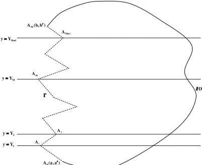
Figure 1: A general domainD and its boundary∂D.
a fixed and a variable part (cure), denoted by Γ. It is joining two known points A = (a, a′) and B = (b, b′) so thata′ ≤ b′ and it makes ∂D simple and closed (see Figure 1). By applying the idea of approximating a curve with broken lines, Γ can be approximated by a finite number of connected segments; we fix this number as M + 1. Therefore, each Γ can be con-sidered as an M + 1 connected segments in which the initial and the final points of them belong to Γ (see Figure 1). If these points are denoted by
A0=A, A1, . . . , AM+1=B,then any appropriate regionD(domain) can be represented by pointsAm= (xm, ym), m= 1,2, . . . , M.
Indeed the variable part of ∂D (and henceD) is represented with 2M vari-ables x1, x2, . . . , xM and y1, y2, . . . , yM. We fix the y-component of each point Am as ym = Ym ∈ R for m = 1,2, . . . , M, so that a′ < Y1 < Y2 <
· · · < YM < b′.0 This would not decries the generalities; since even ym is fixed, but xm is varied and hence Am could be any place on the half line
y(x) =Ym with the vertex on the fixed part of D. Therefore the segments
AmAm+1, m= 0,1, . . . , M, could be selected so that the set of them approx-imates Γ well enough.
Let f ∈C(D×R) and g ∈C(D), be two given real valued functions. The above domainDis called admissibleif the elliptic equation
∆u(X) +f(X, u) =g(X), u|∂D =v, (1) has a bounded solution on the domainD; here it is also supposed thatX = (x, y)∈D,u:D→Ris a bounded trajectory function which takes values in
0 For special case likea′ =b′, one can fix thex-components of points A
m’s instead of
the bounded setU, andv:∂D→Ris a bounded boundary control function, which is Lebesgue measurable and taks values in a bounded set V.
As mentioned, the variable part of ∂D can be approximated with M
number of unknown corners. For a fixed positive integer M, the set of all admissible domains is denoted by DM. When M −→ ∞, if an appropriate optimal shape design problem in DM has a minimizer, then this may tend in some topology to the minimizer over D(the set of all general admissible domains) if such exists. However things can go wrong; for instance: There may be no minimizer overDM; there may be no minimizer overD; or both
D and DM; the sequence of minimizer over DM may not be convergent or may tend in some sense towards a curve that does not define a shape. Young in [24] has shown that their related subsequence of broken lines, tends to an infinitesimal zigzag (generalized curve). This is not (necessarily) an ad-missible curve. So the solution over DM does not tend to the solution over
D, even in the weakly∗-sense. Also, there is the important point that too oscillatory boundaries (like the infinitesimal zigzag) sometimes cause prob-lem; Pironneau in [18] shows some of these problems. Hence, we prefer to fix the number M in this paper, and search for the optimal solution of the appropriate problems overDM.
For a given admissible domain D ∈ DM, let f1 : D×U −→ R and
, f2:∂D×V −→R be two continuous, non- negative, real-valued functions; further, we assume that there is a constant L >0 so that |f1(X, u(X))|≤
L|u|. We define the functional performance criteria, as
I(D, v) =
∫
D
f1(X, u(X))dX+
∫
∂D
f2(s, v(s))ds, (2)
whereuis the bounded solution of (1). We also defineFas the set of all pairs of (D, v) whereD∈ DM andv is the boundary control function. With the above assumption, we are going to solve the following optimal shape design problem onF:
Minimize: I(D, v) =
∫
D
f1(X, u(X))dX+
∫
∂D
f2(s, v(s))ds Subject to: ∆u(X) +f(X, u) =g(X), u|∂D =v, (3) (For some industrial applications of this problem, the reader can have a look on [18]).
To identify the optimal domain inDM, D∗, and its associated optimal control function, v∗D∗, we apply the method which we call shape-measure
optimal pair of domain and its related optimal control function at the same time.
3 Problem in new formulation
In general, even for a fixed domain, it is difficult to characterize a classical bounded solution for the elliptic equation (1). Therefore, one can change the problem into the other form in which a boundedweak(generalized) solution of (1) is involved.
Proposition 1. : Let u be the classical solution of (1), then we have the following integral equality:
∫
D
(u∆ψ+ψf)dX−
∫
∂D
v(▽ψ.n)ds=
∫
D
ψg dX, ∀ψ∈H01(D). (4)
that here nis the outward unit vector on∂D.
Proof. By multiplying (1) with the function ψ ∈ H1
0(D) (the set of functions in the Sobolev space of order 1 in which they are zero on ∂D), integrating overD, and then using the Green’s formula (see [13]), one can obtain the equality (4). □
Now, by regarding [5], letD be a fixed domain; then the mentioned optimal free boundary problem changes into an optimal control one in which the same functional asImust be minimized over the set of all admissible pairs of trajectory and control functions onD. We define Ω =D×Uandω=∂D×V; then, a bounded weak solution and its corresponded control function define a pair of positive and linear functional u(·) :F −→ ∫DF(X, u(X))dX and
v(·) :G−→∫∂DG(s, V(s))dson C(Ω) andC(ω) respectively. As shown in [19] and [20], the Riesz Representation Theorem [21] shows that there are measuresµu andνv so that:
µu(F) =u(F), ∀F ∈C(Ω) ;νv(G) =v(G), ∀F∈C(ω).
So far, we have just changed the appearance of the problem. Indeed the trans-formation between the pair of trajectory and controls, (u, v), and the pair of measures (µu, νv), is injection (see [19]). Now we extend the underlying space and consider the minimization of the problem over the set of all pairs of mea-sures (µ, ν) inM+(Ω)×M+(ω) satisfying the mentioned conditions plus the extra propertiesµ(ξ) =∫Dξ(X)dX =aξ andν(τ) =
∫
∂Dτ(s)ds=bτ; these are deduced from the definition of an admissible pair (u, v) and they indicate that the measures µ and ν project on the (x, y)-plan and real line respec-tively, as Lebesgue measures. We remind the reader that here it is supposed
Therefore, we are going to solve the following problem: Minimize: i(µ, ν) :=µ(f1) +ν(f2)
Subject to: µ(Fψ) +ν(Gψ) =cψ, ∀ψ∈H01(D);
µ(ξ) =aξ, ∀ξ∈C1(Ω);
ν(τ) =bτ, ∀τ∈C1(ω), (5) where Fψ = u∆ψ+ψf , Gψ = −v(▽ψ.n |∂D) and cψ =
∫
Dψg dX. This new formulation has some advantages; for instance, it is linear in respect to the unknown measure, and if we denote Q ⊂ M+(Ω)× M+(ω) as the set of all pairs of measures (µ, ν) satisfying the conditions mentioned in (5), then Qis compact in the sense of the weak∗ topology (see for instance [5]). Moreover the function (µ, ν)∈Q−→µ(f1) +ν(f2)∈Ris continuous. Thus by PropositionII.1 of [19], the problem (5) definitely has a minimizer inQ. The theoretical measure problem (5) is an infinite-dimensional linear program problem; even there is no any identified method for obtaining the solution directly, but its solution can be achieved by choosing the countable sets of functions that are uniformly dense (total), in the appropriate spaces. Let
{ψi : i = 1,2,3, . . .}, {ξj : j = 1,2,3, . . .}, and {τl : l = 1,2,3, . . .}, be total sets in the spaces H01(D),C1(Ω) andC1(ω) respectively. By choosing just a finite number of these functions, the problem (5) is changed into the following one:
Minimize: i(µ, ν) =µ(f1) +ν(f2)
Subject to: µ(Fi) +ν(Gi) =ci, i= 1,2, . . . , M1;
µ(ξj) =aj, j= 1,2, . . . , M2;
ν(τl) =bl, l= 1,2, . . . , M3, (6) where Fi := Fψi, Gi := Gψi, ci := cψi, aj := aξj and bl := bτl. As proved in [5] Theorem 2, the solution of (6) tends to the solution of (5) whenever
M1, M2, M3 −→ ∞; hence the solution of (5) can be approximated by one from (6) when the positive integersM1, M2andM3are chosen large enough. Now one can construct a suboptimal pair of trajectory and control functions for the functionalivia the optimal solution, (µ∗, ν∗), of (6).
4 Atomic measures and discretization
of Rosenbloom’s work which is shown in [19]; by introducing appropriate dense subsets in Ω and ω, one can conclude that µ∗ and ν∗ have the form
µ∗=∑Nn=1αnδ(Zn) andν∗=
∑K
k=1βkδ(zk) whereZn, n= 1,2, . . . , N, and
zk, k = 1,2, . . . , K, belong to dense subsets of Ω andω respectively andδ(t) is the unitary atomic measure with support the singleton set {t}. Hence, by defining a discretization on Ω and ω with the nodes Zn = (xn, yn, un),
n= 1,2, . . . , N, andzk, k= 1,2, . . . , K, the solution of (6) can be obtained by solving the following problem in which its unknowns are the coefficients
αn, n= 1,2, . . . , N, andβk, k= 1,2, . . . , K.
Minimize: N
∑
n=1
αnf1(Zn) + K
∑
k=1
βkf2(zk)
Subject to: N
∑
n=1
αnFi(Zn) + K
∑
k=1
βkGi(zk) =ci, i= 1,2, . . . , M1;
N
∑
n=1
αnξj(Zn) =aj, j= 1,2, . . . , M2; (7)
K
∑
k=1
βkτl(zk) =bl, l= 1,2, . . . , M3;
αn≥0, n= 1,2, . . . , N;
βk ≥0, k= 1,2, . . . , K;. The result of this problem introduces a pair of measures (µ∗, ν∗) that the value of i(µ∗, ν∗), will be minimum; this pair serves the suboptimal pair of trajectory and control functions (uv∗D, v∗D). Thus for the fixed domainD, the minimum value of the functional I in the problem (3) is approximated as I(D, vD∗)≡i(µ∗, ν∗).
5 Searching the optimal curve (domain)
For a given domain, we have explained that how one can find the optimal controlvD∗ for the problem (3), so that the value ofI(D, v∗D) is minimum. To obtain the minimum value of the performance criterionI(D, v) onF, for each domain D ∈ DM, as explained, the variable part of its boundary is defined by a set of points like {Am= (xm, Ym), m= 1,2, . . . , M}. Thus, for a given
D∈ DM, by solving the appropriate finite linear programming problem in (7), the nearly optimal value for I(D, v) (i.e. I(D, vD∗)≡i(µ∗, ν∗)) is calculated as a function of the variables x1, x2, . . . , xM. Consequently, one can define the following function, which is a vector function of variablesx1, x2, . . . , xM:
Now to find the optimal pair of domain (or variable curve) and its related con-trol function inF, say (D∗, vD∗∗), which solves the problem (3), it is enough
to find the minimizer ofJ.
The global minimizer of the vector function J, say (x∗1, x∗2, . . . , x∗M), can be identified by using one of the appropriate standard minimization search meth-ods, like method introduced by Nelder and Mead in [16]; these algorithms usually need an initial set of components (initial domain) to start the process of minimization (we suppose that they give the global minimizer). Each time that the algorithm wants to calculate a value forJ, a finite LP problem like (7) should be solved. Whenever it reaches to the minimum value forJ, the minimizer (x∗1, x∗2, . . . , x∗M) (the optimal curve) and therefore its associated optimal control function have been obtained. So, the optimal domain and its corresponding optimal control are determined at the same time; this is one of the main advantage of this method. Similar to the Proposition 5 of [5], one can easily prove that the method is convergence.
6 Numerical tests
For the following numerical works, we choose a countable total sets of func-tions in each spaces H1
0(D), C1(Ω) and C1(ω), that is, so that the linear combinations of these functions are uniformly dense (dense in the topology of uniform convergence) in the appropriate spaces. We know that the vector space of polynomials with the variablexandy,P(x, y), is dense in C∞(D); therefore the set
P0(x, y) ={p(x, y)∈P(x, y)|p(x, y) = 0,∀(x, y)∈∂D},
is dense (uniformly) in{h∈C∞(D) :h|∂D = 0}≡C0∞(D). Since the set
Q(x, y) ={1, x, y, x2, xy, y2, x3, x2y, xy2, y3, . . .}
is a countable base for the vector space P(x, y), each elements of P(x, y) and also P0(x, y), is a linear combination of the elements in Q(x, y). By Theorem 3 of [13] page 131, the space C∞(D) is dense inH1(D); thus the space C0∞(D) will be dense in H1
0(D). Consequently, the space P0(x, y) is uniformly dense inH1
0(D). Therefore, we define the functionψi for eachias
[6] and [11]) avoids to use the polynomials for such purposes; they usually prefer to apply the related functions defined bysinandcosor combinations of them. To be sure that these polynomials are suitable to determine the shape, we applied them first for determination the inside and the boundary of a circle (as an example of a shape) by applying the embedding method. For this purpose we used the Stock’s theorem for these functions to show the relationship between the inside region and the boundary. The results was very good so that the most obtained inner points (28 from 30) was inside the circle and the rest (two other points) were close enough to the boundary.
For the second set (and also similarly the third one) of functions in (7), letLbe a given positive integer number and divideD intoL(not necessary equal) partsD1, D2, . . . , DL, so that by increasingLthe area of eachDs, s= 1,2, . . . , L,will be decreased. Then, for each s= 1,2, . . . , L, we define:
ξs(x, y, u) =
{
1 (x, y)∈Ds 0 otherwise
These functions are not continuous, but each of them is the limit of an in-creasing sequence of positive continuous functions,{ξsk}; then if µ is any positive Radon measure on Ω, µ(ξs) = limk→∞µ(ξsk). Now consider the set {ξj:j = 1,2, . . . , L} of all such functions, for all positive integerL. The linear combination of these functions can approximate a function in C1(Ω) arbitrary well (see [19] chapter 5).
By definingU =V = [−1.0,1.0] andg(X) = 0, in the following, two examples for the linear and nonlinear cases of the elliptic equations will be presented.
Example 6.1 Let the fixed part of the boundary of D consists of three sides of a unit square joining points A = (1,0),(0,0),(0,1) and B = (1,1); and a variable unknown curve joining points A and B, so that it makes ∂D simple and closed. Therefore qD(x, y) in (9) can be chosen as
xy(y−1)∏Ml=1(x−xl+y−Yl); in this manner,ψi(x, y) is selected so that it is zero on each unknown cornerAm= (xm, Ym) of Γ. Reminding that we are able to choose it in a way that it would be zero on each segment Am−1Am (something which is done in the next example). Now we takef2(s, v) = 0,
f1(X, u) =
{
400 -0.05≤u≤0.05 1
u2 otherwise,
and also M = 8, Y1 = 0.15, Y2 = 0.25, Y3 = 0.35, Y4 = 0.45, Y5 = 0.55,
Y6= 0.65,Y7= 0.75,Y8= 0.85. The control function is supposed to be zero on∂Dexcept the segment of liney= 1 which along this segment,v(s) takes values inV, whens∈[0,1]. Thus, in (7) we haveGi=−(∂ψi(s,y)∂y )|y=1.
To set up the finite linear programming (7) for the next two cases, we choose
dis-cretization on Ω with N = 1100 nodes by points Zn = (xn, yn, un), n = 1,2, . . . , N. Because the control function is zero on∂D except the segment of the liney= 1, we have put a discretization onωwithK= 110 nodes like
zk = (sk, vk), k= 1,2, . . . , K; these nodes have been chosen aszk =z11(i−1)+j for i = 1,2, . . . ,10 and j = 1,2, . . . ,11, where s11(i−1)+j =
(i−1)+0.5 10 and
v11(i−1)+j = 2(j−1)
10 −1.0. Hence the total number of variables in a simi-lar problem to (7) is 1100 + 110 = 1210. In the case of these concepts, we solved the following examples for the linear and nonlinear case of the ellip-tic equations; in each case we chose the subroutine AM OEBA (see [17]) as the standard minimization algorithm with the initial valves Xm = 1.0, for
m= 1,2, . . . ,8 (indeed, here the initial domain is selected as a unit square). Also, we applied theE04M BF NAG-Library Routine for solving the appro-priate finite linear program.
Linear Case: In this example for the linear case, we chosef = 0; then by applying the mentioned method, after 497 iteration we achieved the optimal value ofI = 0.44432256772971. The value of the variables in the final step was
X1= 0.044671, X2= 0.000003, X3= 0.000018, X4= 0.083868, X5= 0.004590,
X6= 1.181268, X7= 0.003360, X8= 1.291424.
According to the obtained results, the suboptimal control function, the initial and the final domain, and also the changes diagram of the objective function according to the number of iterations, have been plotted in the Figures 2, 3 and 4. We remind that one could do some smoothness and get better results (see Example 6.2 for instance).
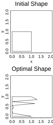
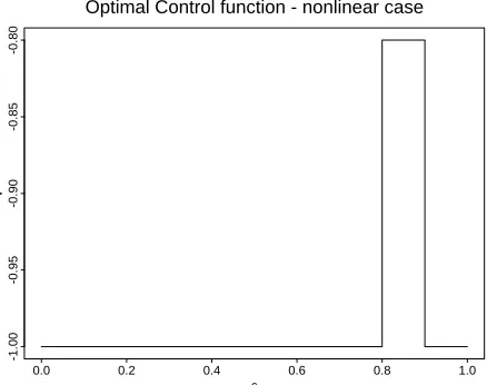
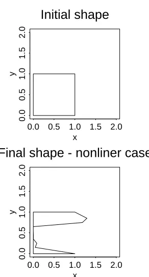
Nonlinear case: By choosingf = 5u2 and applying the other assumption as above, the example for the nonlinear case of the elliptic equations was solved. After 492 iterations, the optimal value was I = 0.44432182922939 and the value of the variables in the final step was X1 = 0.044691, X2 = 0.083889, X3= 0.004568, X4= 0.003356, X5= 0.000026, X6= 0.000001, X7= 1.181291, X8= 1.291379. The results have introduced the suboptimal control function, the final domain and the changes diagram of the objective function which have been plotted in the Figures 5, 6 and 7.
Example 6.2 Let the fixed part of the boundary be the left half of the unite circle, joining the pointsA= (0,−1) andB= (0,1). Hence forM = 9,
qD(x, y) in (9) can be chosen as
(x+√1−y2)(x−5X1(y+1))(x−5X9(y−Y9)) 9
∏
l=2
(x−Xl−1−5(Xl−Xl−1)(y−Yl−1)),
where Y1 = −0.8, Y2 = −0.6, Y3 = −0.4, Y4 = −0.2, Y5 = 0, Y6 = 0.2,
s
v
0.0 0.2 0.4 0.6 0.8 1.0
-1.0
-0.5
0.0
0.5
1.0
Optimal Control function - linear case
Figure 2: The optimal boundary control function for the linear case of Ex-ample 6.1.
x
y
0.0 0.5 1.0 1.5 2.0
0.0
0.5
1.0
1.5
2.0
Initial Shape
x
y
0.0 0.5 1.0 1.5 2.0
0.0
0.5
1.0
1.5
2.0
Optimal Shape
iteration
value
0 100 200 300 400 500
0.6
0.8
1.0
•
•
•
•
• •
• • • • •
Changes of Objective function - linear case
Figure 4: Change of the objective function according to iterations for the linear case of of Example 6.1.
s
v
0.0 0.2 0.4 0.6 0.8 1.0
-1.00
-0.95
-0.90
-0.85
-0.80
Optimal Control function - nonlinear case
x
y
0.0 0.5 1.0 1.5 2.0
0.0
0.5
1.0
1.5
2.0
Initial shape
x
y
0.0 0.5 1.0 1.5 2.0
0.0
0.5
1.0
1.5
2.0
Final shape - nonliner case
Figure 6: The initial and the optimal domain for the nonlinear case of Ex-ample 6.1.
iteration
value
0 100 200 300 400 500
0.6
0.8
1.0
•
•
•
•
• • •
• • • •
Change of the objective function - nonlinear case
0.5
-0.47
-0.48
-0.49
3
-0.5
-0.51
2.5
-0.52
-0.53
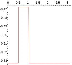
2 1.5 1 0
Figure 8: The optimal boundary control function for the linear case of Ex-ample 6.2.
we have Gi = v
√
1−y2ψ
ix−vyψiy. To show that the method is suitable enough even for the hard situations, we considered much more difficulties in conditions. Therefore, it is supposed that here the variables xi’s have an upper bounds √1−Y2
i and a lower bound which guaranteed that the variable points can not pass the left half of the unite circle. These conditions are applied by means of the penalty method (see [22]). By selecting
f2(s, v) =
{ √
(Xi+ 5(Xi−Xi−1)(s−Yi−1)2+s2,Yi−1≤s≤Yi
s2−v2−1, 1≤s≤1 +π,
K = 3200, N = 11875, M2 = 9 and M3 = 15 (9 equation for fixed bound-ary and the rest for Γ), an extra condition for the summation of αi’s is also considered to be sure that the domain is covered by characteristic functions perfectly. Thus Ω and ω are discretized by 15075 nodes in which 100 of them was chosen from the fixed part of boundary and also on each segment
Am−1Am, 20 nodes was selected. Moreover the subroutinesAM OEBA and
DLLRRS from the Fortran library were used for solving the following exam-ples.
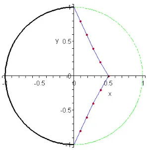
Linear Case: Let f1 = 1−u2 and f = 0 (hence the elliptic equation (1) is linear). The initial domain is selected as complete unite circle. After 785 iterations, the optimal value was converge to 19.9850134 and the optimal val-ues ofxi’s were: 0.941, 0.1868, 0.2767, 0.3863, 0.5033, 0.3845, 0.2770, 0.1870, 0.0945. The nearly optimal control and the optimal domain, before and after fitting a smooth curve by means of the natural cubic Spline, were plotted in Figures 8, 12 and 10 (by use of Maple9.5 software).
Figure 9: The optimal domain for the linear case of Example 6.2 before fitness.
0.5 1
0
-0.5
3 2.5 2 1.5 1 0
0.5
Figure 11: The optimal boundary control function for the nonlinear case of Example 6.2.
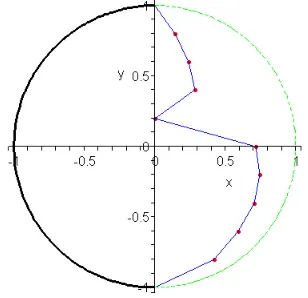
Figure 12: The optimal domain for the nonlinear case of Example 6.2 after fitness.
also selected as a unit circle and after 1303 iterations the optimal control and the optimal domain are obtained. The optimal control is plotted in Figure 11 and after fitting a smooth curve as above, the optimal domain for this case is shown in Figure 12. In this case, the optimal value was 10.699029.
7 Conclusions
control function simultaneously; moreover, the optimal value for the general form of the objective function were determined in an easy way just by apply-ing a standard search technique and also the simplex algorithm perfectly well. Presenting a linear treatment even for the extremely nonlinear problems was one of the main advantages of this method.
Acknowledgements
The author is very grateful to Prof. Rubio for his valuable comments and all his help.
List of symbols D: a domain
∂D: boundary of D
u: solution of the elliptic system
v: boundary control
DM: the set of admissible domains for fixed M
D: the set of general admissible domains F: the set of all pairs of (D, v) whereD∈ DM n: is the outward unit vector on∂D
H1(D): the Sobolev space of order 1
H1
0(D): set of functions inH1(D) in which they are zero on∂D
C(Ω): the set of continuous and bounded functions on Ω
C1(Ω): the set of functions inC(Ω) which depend only on the first variable
M+(Ω): the space of positive Radon measures onC(Ω)
P(x, y): the space of polynomials ofxandy.
References
1. Alt, W. and Dembo, M.Cytoplasm dynamics and cell motion: two-phase flow models, Int. J. Mathematical Biosciences, 156 (1999), 207–228. 2. Berger, M. P. F. and Wong, W. K.Apllied Optimal Designs, John Wiley
& Sons Ltd, 2005.
3. Fakharzadeh Jahromi, A. and Rubio, J. E.Shapes and Measures, Journal of Mathematical Control and Information, 16 (1999), 207-220.
5. Fakharzadeh Jahromi, A. and Rubio, J. E.Best Domain for an Elliptic
Problem in Cartesian Coordinates by Means of Shape-Measure, AJOP
Asian J. of Control, 11, 5 (2009), 536–547.
6. Farahi, M. H.The Boundary Control of the Wave Equation, PhD thesis, Leeds University (1996).
7. Goberna, M. A. and Lopez, M. A. Linear Semi-infinite Optimization, Alicant Uiniversity, 1998.
8. Hadamard, J.Lessons on the Calculus of Variation. Gauthier-Villards, Paris, 1910. (in French).
9. Haslinger, J. and Neittaanamaki, P. Finite Element Approximation for Optimal Shape Design: Theory and Applications, Johan Wiley & Sons Ltd, 1988.
10. Haug, E. J. and Cea, J. Optimization of Disstributed Parameter Struc-tures, Vols I and II, Sijthoff and Noordhoff, Alpen and Rijn, The Nether-land, 1981.
11. Kamyad, A. V., Rubio, J. E. and Wilson, D. A. The optimal control of multidimensional diffusion equation, JOTA, 1, 70 (1991), 191–209. 12. Lancaster, K. E.Qualitative behavior of solution of elliptic free boundary
problems, Pacific J. Maths., 154, 2 (1992), 297–317.
13. Mikhailov, V. P.Partial Differential Equation, MIR Publisher, Moscow, 1978.
14. Munch, A.Optimal design of the support of the control for the 2-d wave
equation: Numerical investigation, Mathematical Modeling and
Numer-ical Analysis, 5, 2 (2008), 331–351.
15. Munch, A.Optimal internal dissipation of a damped wave equation using a topological approach, Int. J. Appl. Math. Comput. Sci., 19, 1 (2009), 15–37.
16. Nelder, J. A. and Mead, R.A simplex method for function minimization, The Computer Journal, 7 (1964-65), 303-313.
17. Press, W. H.,Teukolsky, S. A., Vetterling, W. T. and Flannery, B. R.
Neumerical Recipes in Fortran: The art of scientific computing, 2ed edi-tion, Cambridge unversity press, 1992.
18. Pironneau, O. Optimal Shape Design for Elliptic System, Springer-Verlag, New York - Berlin - Heidelberg - Tokyo, 1983.
20. Rubio, J. E.The global control of nonlinear elliptic equation. Journal of Franklin Institute, 330, 1 (1993), 29–35.
21. Rudin, W. Real and Complex Analysis, Tata McGraw-Hill Publishing Co.Ltd, New Delhi, second edition, 1983.
22. Sun, W. and Ya-Xiang, X.Optimization Theory and Methods: Nonlinear programming, Springer, 2006.
23. Vogel, T.A free boundary problem arising from galvanizing process, SIAM J. Math. Mech. Anal., 16 (1985) 970–979.
24. Young, L. C.Lectures on the Calculues of Variations and Optimal Control