Volume 30 - Article 27 | Pages 795–822

(1)

DEMOGRAPHIC RESEARCH

VOLUME 30, ARTICLE 27, PAGES 795–822

PUBLISHED 14 MARCH 2014

http://www.demographic-research.org/Volumes/Vol30/27/ DOI: 10.4054/DemRes.2014.30.27

Research Article

Joint probabilistic projection of female and

male life expectancy

Adrian E. Raftery

Nevena Lalic

Patrick Gerland

c

2014 Adrian E. Raftery, Nevena Lalic & Patrick Gerland.

(2)

2 Data 798

3 Methodology 801

3.1 Review of the one-sex Bayesian hierarchical model for life expectancy 801

3.2 Modeling the gap 802

4 Model validation 806

4.1 Projections of male and female life expectancy 808

5 Country-specific case studies 809

5.1 Ireland 809

5.2 Guatemala 810

5.3 Laos 811

5.4 Cambodia 812

6 Discussion 814

7 Acknowledgements 816

(3)

Joint probabilistic projection of female and male life expectancy

Adrian E. Raftery1

Nevena Lalic2

Patrick Gerland3

Abstract

BACKGROUND

The United Nations (UN) produces population projections for all countries every two years. These are used by international organizations, governments, the private sector and researchers for policy planning, for monitoring development goals, as inputs to economic and environmental models, and for social and health research. The UN is considering pro-ducing fully probabilistic population projections, for which joint probabilistic projections of future female and male life expectancy at birth are needed.

OBJECTIVE

We propose a methodology for obtaining joint probabilistic projections of female and male life expectancy at birth.

METHODS

We first project female life expectancy using a one-sex method for probabilistic projec-tion of life expectancy. We then project the gap between female and male life expectancy. We propose an autoregressive model for the gap in a future time period for a particular country, which is a function of female life expectancy and at-distributed random pertur-bation. This method takes into account mortality data limitations, is comparable across countries, and accounts for shocks. We estimate all parameters based on life expectancy estimates for 1950-2010. The methods are implemented in the bayesLife and bayesPop R packages.

1_{A. E. Raftery, Departments of Statistics and Sociology, University of Washington, Seattle, Washington, USA.}

Correspondence to Adrian E. Raftery, Department of Statistics, Box 354322, University of Washington, Seattle, WA 98195-4322, USA. E-Mail: [email protected].

2_{N. Lalic, Institutional Research, University of Washington, Seattle, Washington, USA.}

3_{P. Gerland, United Nations Population Division, Population Estimates and Projection Section, New York, New}

(4)

RESULTS

We evaluated our model using out-of-sample projections for the period 1995-2010 and found that our method performed better than several possible alternatives.

CONCLUSIONS

We find that the average gap between female and male life expectancy has been increasing for female life expectancy below 75, and decreasing for female life expectancy above 75. Our projections of the gap are lower than the UN’s 2008 projections for most countries and thus lead to higher projections of male life expectancy.

1. Introduction

Every two years, the Population Division of the United Nations (UN) publishes theWorld

Population Prospects(WPP), reporting population estimates and projections for all

coun-tries. Experts then use these projections to monitor population trends and as inputs to economic and environmental models. The UN’s population projections form the basis of many nations’ and regions’ development plans (Heilig et al. 2010).

Since 1980, each edition of the WPP has included three projection variants: low, medium, and high. The medium variant is intended to represent the most likely population size given past trends and expert knowledge. The low and high variants are then generated using different fertility assumptions: total fertility is taken to be half a child either below or above that used to generate the medium scenario. Thus the variation in fertility allowed by this method is insensitive to either the level of fertility in a particular country or its trend. The assumptions about mortality and international migration are the same in all three variants.

Deterministic population projections are unable to take into account the full variabil-ity in demographic processes across countries or to indicate a range of future population outcomes. As a result, the UN is considering issuing probabilistic population projections as an alternative to their standard variants of deterministic projections. As WPP projec-tions are based on the cohort-component method, probabilistic projecprojec-tions of the main de-mographic processes affecting national populations (fertility, mortality and international migration) are required to produce probabilistic population projections for all countries.

Probabilistic projections of fertility for all countries have already been developed by Alkema et al. (2011) and implemented in WPP 2010 (United Nations 2011). The medium variant in WPP 2010 corresponds to the median of the many possible future fertility paths for each country generated by the Alkema et al. (2011) model.

(5)

fore-casting mortality is to project life expectancy and use either recent mortality patterns or model life tables to obtain the age pattern required for use in cohort-component meth-ods (Booth 2006). Given the missing and frequently inaccurate data available for many countries, this method is used by the UN for most countries.

A probabilistic approach to projecting life expectancy for males has been developed by Raftery et al. (2013) and is an extension of the UN’s current method. It models life expectancy in a country as a random walk with a nonconstant drift, where the drift term is a nonlinear function of current life expectancy and reflects varying rates of improvement for countries at different levels of life expectancy. The use of a Bayesian hierarchical model (BHM) allows for the estimation of the rate of improvement in life expectancy for a country using past data from that country, while also taking into account observed patterns in other countries. The same model can be used for female life expectancy.

The BHM of Raftery et al. (2013) has the disadvantage that it models life expectancy for one sex only, and disregards the relationship between male and female life expectan-cies. Thus, like many other mortality forecasting models (Bongaarts 2009; Cairns et al. 2011; Haberman and Renshaw 2008; Hyndman and Shahid Ullah 2007; Shang, Booth, and Hyndman 2011; Soneji and King 2011), it does not producejointprojections of male and female life expectancy. These are required to obtain fully probabilistic projections of life expectancy for both sexes and to avoid crossovers that are not expected to occur in the future. Girosi and King (2008) proposed a general approach to projecting age-specific mortality rates that could, in principle, be used for this problem, but they did not describe an explicit method for doing so.

Li and Lee (2005) have proposed a method for forecasting mortality for both sexes in a country using the augmented common factor model, which is a general method for achieving coherence between the mortality rates of different groups (in this case the two sexes in a population) that are expected not to diverge. Hyndman, Booth, and Yasmeen (2013) extended this to model the smoothness of mortality rates explicitly with respect to age, using the product-ratio functional method.

Here we propose a method for joint probabilistic projection of male and female life ex-pectancy that ensures coherence between them in a simple manner: by projecting the gap between them. The gap is defined as female life expectancy minus male life expectancy, and is thus positive in most cases. Projections of female life expectancy are generated by the BHM, and are then combined with projections of the gap to produce projections of male life expectancy.

(6)

addition, many have commented on the recent narrowing of the gap in high-income coun-tries (Bobak 2003; Conti et al. 2003; Emslie and Hunt 2008; Glei and Horiuchi 2007; Gómez-Redondo and Boe 2005; Kołodziej, Łopusza´nska, and Jankowska 2008; Meslé 2004; Pampel 2005; Preston and Wang 2006; Trovato and Lalu 1996; Trovato and Ody-nak 2011; Staetsky 2009; Staetsky and Hinde 2009).

While several authors have provided opinions about the probable trajectory of the gap in high-income countries (Meslé 2004; Rogers et al. 2010; Trovato and Lalu 2007), few have attempted to make explicit projections (Pampel 2005; Preston and Wang 2006). When they did so, they focused on data-rich high-income countries. We are aware of only two studies that study the gap in life expectancy in developing countries: They show that conflicts (Plümper and Neumayer 2006) and natural disasters (Neumayer and Plümper 2007) have different effects on the life expectancy of the two sexes, and thus affect the gap between them.

We propose to model the gap in life expectancy between females and males for all the countries that are not in the midst of a generalized HIV/AIDS epidemic. After briefly discussing the data we use, we describe the model. Next, we assess the performance of our model and possible competing models using data from 1950-1995 to project life expectancy over the period 1995-2010. We then discuss our projections for four countries chosen as examples of possible future trends in the gap between female and male life expectancy: continued decline in the gap for a country in which the decline has already been observed (Ireland), decline in the gap for a country in which the decline has not yet been observed (Guatemala), continued rise, followed by a decline (Laos), and continued rise over the projection period (Cambodia). We conclude with a discussion of the merits and limitations of our method.

2. Data

We use the WPP 2008 estimates of past life expectancy from 1950 to 2010 for all the countries in the world (United Nations 2009). We compare our projections with the WPP 2008 projections of life expectancy for the period 2010-2050. These data and projections are included in the R packagewpp2008(Ševˇcíková and Gerland 2014).

(7)

Mortality patterns are significantly affected by the HIV/AIDS epidemic, which has been a major source of mortality in the last twenty years and has predominantly affected young or middle-aged adults, unlike most other causes of death. As a result, we exclude countries with a generalized HIV/AIDS epidemic, as defined by the Joint United Nations Programme on HIV/AIDS (UNAIDS). We also exclude small countries with a population of 100,000 or less. Thus we concentrate on 158 countries with 100,000 inhabitants or more and no generalized HIV/AIDS epidemic. In 2009 these accounted for 89.2% of the world population.

The data for male and female life expectancy at birth in these 158 countries for the pe-riod 1950-2010 are shown in Figure 1. We note several patterns: both male and female life expectancy at birth have been increasing over time, with median female life expectancy in the last period (76.5 years) being higher than male (70.9 years). The between-country variability has decreased over time. The median gap between female and male life ex-pectancy increased from 1950-1955 to 1990-1995, with a slight decline thereafter.4 In 2005-2010, the median gap in life expectancy was 4.9 years, with an interquartile range of (3.9, 6.6). The between-country variability in the gap in life expectancy has declined over time. However, in each quinquennium, at least one country had a gap that was ex-treme relative to the other countries. The presence of outliers must thus be taken into account when projecting the gap in future periods.

Figure 1: Trends in male and female life expectancy at birth (e0) and the gap

between them for all 158 countries under study over the period 1950–2010, based on estimates in WPP 2008

30 40 50 60 70 80 90 Ma le e0

1953 1958 1963 1968 1973 1978 1983 1988 1993 1998 2003 2008

30 40 50 60 70 80 90 F ema le e0

1953 1958 1963 1968 1973 1978 1983 1988 1993 1998 2003 2008

-5 0 5 10 15 Gap in e0

1953 1958 1963 1968 1973 1978 1983 1988 1993 1998 2003 2008

Notes: The dark lines in the boxplots indicate median values, the gray boxes extend to the first and third quartile,

and the whiskers extend to the most extreme data point which is no more than 1.5 times the interquartile range from the box. Each quinquennium is identified by its middle year (e.g. 1950–1955→1953).

4_{In WPP, vital events and associated rates refer to five-year periods from mid-July to mid-July. Thus, for}

(8)

Figure 2 displays the narrowing of the gap in life expectancy between the sexes that has been reported in the literature for high-income countries. We use membership of the Organization for Economic Cooperation and Development (OECD) as a distinguishing trait. The trend is not present in non-OECD countries, though some, including Brazil and Uruguay, have experienced lower levels of the gap at higher levels of female life expectancy. Figure 2 also shows that the trend in the gap is more easily seen when plotted against female life expectancy than against time.

Figure 2: Trends in the gap between female and male life expectancy at birth for OECD (right panels) and non-OECD countries (left panels) over time (top panels) and over female life expectancy at birth (bottom panels) for 1950-2010 as reported in WPP 2008

1960 1970 1980 1990 2000 2010

-5 0 5 10 15 20

non-OECD Countries by Year

Year Gap in e0 Uruguay Brazil Bhutan

1960 1970 1980 1990 2000 2010

-5 0 5 10 15 20

OECD Countries by Year

Year

Gap in

e0

United States Italy

30 40 50 60 70 80 90

-5 0 5 10 15 20

non-OECD Countries by Female e0

Female e0

Gap in

e0

Uruguay Brazil

Bhutan

30 40 50 60 70 80 90

-5 0 5 10 15 20

OECD Countries by Female e0

Female e0

Gap in

e0

United States _Italy

Notes: The red lines show a loess smooth of the data points. The trend in the gap for five countries is shown for

(9)

3. Methodology

Until the 2010 revision of theWorld Population Prospects, the UN projected female and male life expectancy independently and deterministically, using point forecasts from the method of Lee and Carter (1992), with a modification to ensure that projections for the two sexes do not diverge (Li and Lee 2005).

3.1 Review of the one-sex Bayesian hierarchical model for life expectancy

The BHM of Raftery et al. (2013), which we now briefly summarize, is a one-sex model. Female life expectancy at birth for countryc in five-year periodt, denoted byef₀_,c,t, is assumed to follow a random walk with drift, given by

ef₀_,c,t₊₁=ef₀_,c,t+g(ef₀_,c,t|θ(c)) +εc,t+1, (1)

whereεc,t ind

∼ N(0, ωf(ef₀_,c,t)), withf(ef₀_,c,t)a smooth declining function ofef₀_,c,t. In equation (1), the expected five-year gain in life expectancy is a double-logistic function of the current level of life expectancy, namely

g(ef₀_,c,t|θc) = k

c

1 + exp(−A1 ∆c 2

(ef_c,t−∆c

1−A2∆c2)) +

zc₋_kc

1 + exp(−A1 ∆c

4(e f ct−

P3

i=1∆ci−A2∆c4))

, (2)

whereθc _{= (∆}c

1,∆c2,∆c3,∆c4, kc, zc)are the six parameters of the double-logistic

func-tion for countryc, andA1andA2are constants.

Each of the parameters of the double-logistic function for countrycis in turn assumed to be drawn from a world distribution of the parameter:

∆c_i|σ∆i iid

∼ Normal[ai,bi](∆i, σ2∆i), i= 1, . . . ,4, (3)

kc|σk iid

∼ Normal[0,10](k, σk2), (4)

zc|σz iid

∼ Normal[0,1.15](z, σz2), (5)

where Normal[a,b](µ, σ2)denotes a normal distribution with meanµand standard

(10)

3.2 Modeling the gap

To obtain joint probabilistic projections of female and male life expectancy, we need to model the relationship between the two. We do this by projecting the gap in life ex-pectancy by linear regression using female life exex-pectancy as a covariate.

The pattern of decline in the gap in life expectancy has been observed only for high-income countries, and for some emerging economies. The question then arises: should we project that other countries will also follow this pattern? Vallin (2006) argued that there is no reason why the experience of English-speaking countries and Scandinavian countries (now extended to most high-income countries) should not become generalized, enabling men in most places to eventually regain some of the ground they lost during the 20th cen-tury. Bongaarts (2009) agreed that mortality patterns observed for high-income countries will most likely be followed by others: “There is an expectation that, as developing coun-tries evolve, they will also get rid of non-senescent mortality, since non-senescent deaths unrelated to aging (e.g., accidents, certain infections) can be avoided by effective public health and safety measures and through medical intervention.”

We note also in Figure 2 that non-OECD countries have much lower female life ex-pectancy than OECD countries, and it is only at high levels of female life exex-pectancy that a narrowing in the sex gap has been observed. Thus, it is plausible that the reversal has not yet been seen in most non-OECD countries simply because they have not yet reached the female life expectancy level at which the gap begins to narrow.

Between 1950 and 2010, several countries experienced events that have had a signif-icant impact on the gap between female and male life expectancy. The gap in Bosnia and Herzegovina increased gradually from 2.2 to 5.3 years between 1950-1955 and 1985-1990, then jumped to 17.3 years in 1990-1995 during a period of conflict, before falling to 5.4 years in the next quinquennium. Similarly, the gap in Iraq increased from 6.3 years in 1980-1985 to 12.7 years in 1985-1990, and remained at approximately that level until the 1995-2000 quinquennium, when it dropped to 5.6 years. Because we can expect such shocks to continue in the future, we must allow for outliers in our model.

Ours is not the first attempt to deal with outliers in mortality data. Hyndman and Shahid Ullah (2007) used robust statistics in developing their method for forecasting age-specific mortality and fertility rates observed over time. However, while their objective was to identify and remove data associated with extreme events, ours is to incorporate them in our projections so as to capture perturbations that may occur in the future more realistically.

(11)

We found that thet-distribution tended to generate outliers similar qualitatively to those observed in the data, but also occasionally generated very large outliers of much greater magnitude than any observed in the data. As a result, we truncated the predictive distri-bution, with the truncation points estimated from the data. This gave a model that yielded outlying values of the gap similar to those observed historically, but not very extreme outliers beyond the range of experience.

To produce joint probabilistic projections of female and male life expectancy, we project the gap in life expectancy by simulating a large number of future trajectories from a linear regression model with BHM female life expectancy projections as a covariate. For each simulated value of the gap, we subtract it from a simulated value of female life expectancy projection to obtain the corresponding simulated male life expectancy projection. The result is a large number of (female e0, male e0) pairs, which form a

sample from the joint predictive distribution sought.

We use female rather than male life expectancy as a basis for projecting the gap be-cause female life expectancy tends to be more stable and more accurately measured. For comparison purposes, however, we also build a model for the gap using male life ex-pectancy projections from the BHM for comparison.

Our proposed model for the gap in life expectancy at birth between females and males represents the gap,Gc,tfor countrycin the current quinquennium,t, as a linear combina-tion of four terms. These are: the gap in the previous quinquennium,Gc,t−1; female life

expectancy at birth in the first quinquennium in our dataset (1950-1955),ef₀_,c,₁₉₅₃; female

life expectancy at birth in the current quinquennium,ef₀_,c,t; and the number of years by

whichef₀_,c,t exceedsτ, namely(ef₀_,c,t−τ)+, where we use the notation(x)+ = xif

x > 0and 0 otherwise. The quantityτ is the level of female life expectancy at which the gap is expected to stop widening and to start narrowing. Finally, at the highest ob-served levels of female life expectancy and beyond, denoted by agesAand greater, the gap is modeled as a random walk with normally distributed changes and no drift. This is because we have little information on the determinants of changes in the gap at these high ages and we have observed no outliers for the countries with the highest current life expectancies.

In summary, our model is as follows:

Gc,t= min{max{G∗c,t, L}, U},

where

G∗_c,t= 

 

 

β0+β1ef0,c,1953+β2Gc,t−1+β3ef0,c,t+ β4(e

f

0,c,t−τ)++ε (1)

c,t, ife

f

0,c,t≤A, Gc,t−1+ε

(2)

c,t, ife

f

(12)

where

ε(1)_c,t iid∼ t(µ= 0, σ(1)2, ν= 2),

ε(2)_c,t iid∼ N(0, σ(2)2).

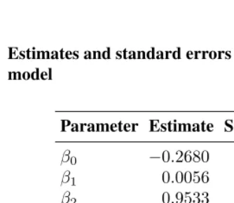
Estimates of the parameters of this model based on data from 158 countries for 1950-2010 contained in WPP 2008 were obtained by maximum likelihood and are reported in Table 1. The maximum likelihood estimates ofLandU are the minimum and maximum observed gaps respectively, namelyLˆ = −2.67andUˆ = 17.34. Given these values, all theG∗

c,t for the historical data period are observed. Conditionally onτ andA, the model for theG∗

c,t is thus a linear regression model with truncatedt-distributed errors, and we estimated it from the historical data by approximate maximum likelihood using the R packagehett(Taylor 2009). The approximation arises from the fact that the full likelihood involves a factor due to the truncation that we ignore; numerical experiments indicated that including this would make little difference to the results. We then maxi-mized the resulting maximum likelihoods over integer values ofτandAto obtain overall maximum likelihoods. The resulting estimates wereτ = 75years andA =83 years. While slight heteroscedasticity was observed, we chose not to model it explicitly so as to keep the model as simple as possible. Also, the original estimate of the degrees of freedom parameter was 2.07 (standard error 0.13), which we rounded down to 2, again for simplicity.

Table 1: Estimates and standard errors of parameters used in gap projection model

Parameter Estimate Standard Error

β0 −0.2680 0.0648

β1 0.0056 0.0011

β2 0.9533 0.0044

β3 0.0056 0.0013

β4 −0.0851 0.0053

σ(1) ₀_.₂₅₇₂

σ(2) ₀_.₄₁₉₉

τ 75

A 83

L −2.67

(13)

This model represents the empirical regularities in the data in a simple way. The gap in five-year periodt,Gc,t depends on the gap in periodt−1,Gc,t−1, reflecting the fact

that the gap evolves over time in a somewhat smooth way. Our estimate ofβ2was highly

significantly positive and our estimate of β4 was highly significantly negative, withp

values less than10−5_{in both cases. Thus the gap increases with female life expectancy}

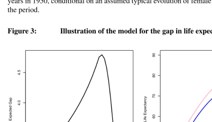
for female life expectancy up to about age 75, and decreases thereafter up to about age 83; this reflects the pattern seen in the lower right panel of Figure 2. Beyond that our data are too sparse to provide evidence for anything other than a random walk without drift. The model is illustrated in Figure 3, showing the expected evolution of the gap over 150 years from 1950 to 2100, for a country with female life expectancy at birth of 40 and a gap of 3 years in 1950, conditional on an assumed typical evolution of female life expectancy over the period.

Figure 3: Illustration of the model for the gap in life expectancy

40 50 60 70 80 90

3.0

3.5

4.0

4.5

Female Life Expectancy

Exp

ect

ed

G

ap

1950 2000 2050 2100

40

50

60

70

80

90

Year

Li

fe

Exp

ect

an

cy

Female Male

Notes: Left panel: Expected evolution of the gap in life expectancy as a function of female life expectancy. Right

panel: Expected evolution of female and male life expectancy over the period 1950–2100. Both are for a hypothetical country with female life expectancy at birth of 40 and a gap of 3 years in 1950, conditional on an assumed typical evolution of female life expectancy over the period.

(14)

corresponds roughly to the demographic transition involving decreasing fertility, so this may be one factor explaining the initial increase in the gap.

In populations with medium life expectancy, men are typically exposed to higher risk than women in midlife, such as dangerous physical jobs and riskier lifestyles (smoking, drinking, physical risk-taking), leading to a higher gap in life expectancy. In countries with high life expectancy, infant and child mortality is low for both sexes and hence quite similar for males and females, and differences in life expectancy are due at least partly to different lifestyles of men and women (Gjonça, Tomassini, and Vaupel 1999; Waldron 1995). These lifestyles may become more similar over time, partly explaining why the gap in life expectancy is closing past a certain level of longevity.

Beyond female life expectancy ofA = 83years, our model does not project further linear declines in the gap, as we have few data on which to base projections. A contin-ued decline in the gap would imply that the gap would eventually become negative in all countries, with high probability. However, several authors have noted that there may be biological reasons why this would be unlikely (Austad 2011; Soliani and Lucchett 2006; Vallin 2006), including the protective effect of oestrogen (Lord et al. 2010), adverse ef-fects of testosterone (Bassil and Morley 2010), and women’s more robust immune systems (Owens 2002; Falagas, Vardakas, and Mourtzoukou 2008).

The overall level of the gap is also positively related to female life expectancy at the beginning of our data in 1950. Finally, this is a linear regression model withtdistributed errors. Thet distribution has longer tails and generates more outliers than the normal distribution, and so this model allows for the occasional extreme values that we observe in the data.

The overall method for joint probabilistic projection of female and male life ex-pectancy is implemented in the bayesLife R package (Ševˇcíková and Raftery 2014), for which a GUI is provided by the bayesDem R package (Ševˇcíková 2013).

4. Model validation

In order to assess the performance of our model, we estimated model parameters based on the data from 1950 to 1995 only, containing 1,422 country-period combinations, and we then forecast the gap in life expectancy from 1995 to 2010. We then compared our results to WPP 2008 estimates of the gap for those three quinquennia. This yielded 474 out-of-sample projections.

(15)

makes small errors in prediction). We measured accuracy by reporting the mean absolute error of the median of the probabilistic projections.

We also compared the performance of our model to other potential gap projection methods. For the gap in life expectancy, we compared the performance of the gap model based on female life expectancy to the gap model based on the male life expectancy, as well as to the difference between independent projections of female and male life ex-pectancy under the BHM, constrained to the range[−3,18](“BHM Projection”). We also report the accuracy of a model that assumes that the gap would remain at 1990-1995 levels from 1995 to 2010 (“Constant 1995 Gap”). Our results are shown in Table 2.

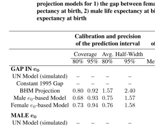
Table 2: Results for 15-year out-of-sample cross-validation for four different projection models for 1) the gap between female and male life ex-pectancy at birth, 2) male life exex-pectancy at birth, and 3) female life expectancy at birth

Calibration and precision Accuracy of the prediction interval of the prediction

Coverage Avg. Half-Width

80% 95% 80% 95% Mean Absolute Error

GAP INe0

UN Model (simulated) – – – – 0.78

Constant 1995 Gap – – – – 0.73

BHM Projection 0.80 0.92 1.57 2.40 0.78

Malee0-based Model 0.68 0.93 0.75 1.57 0.70

Femalee0-based Model 0.73 0.94 0.76 1.58 0.66

MALEe0

Constant 1995 Gap 0.64 0.85 1.61 2.46 1.42

BHM Projection 0.79 0.94 2.05 3.13 1.44

Gap-based Model 0.76 0.93 1.90 3.02 1.32

FEMALEe0

Constant 1995 Gap 0.86 0.96 2.05 3.14 1.14

BHM Projection 0.75 0.90 1.61 2.46 1.16

Gap-based Model 0.89 0.97 2.23 3.48 1.17

(16)

had good coverage and precision, and provided the most accurate projections among the models that we considered. In comparison, the BHM projection of male life expectancy had good coverage, but it had low precision, particularly the 80% prediction interval, which was more than twice as wide on average as that of the other two models. It was also 11–18% less accurate than the other two models. The gap model based on male rather than female life expectancy had worse coverage and was less accurate than the female-based model.

4.1 Projections of male and female life expectancy

Next we used our projections of the gap and the BHM projections of female life ex-pectancy to generate projections of male life exex-pectancy, and we performed the same cross-validation exercise. We compared our results to three other sets of projections:

(1) Projections prepared for 1995-2010 with the current standard methods of deter-ministic projection of life expectancy used in the WPP. These used one of the five prescribed UN models of gains in life expectancy at birth used in the 2008 WPP based on levels and trends during 1985-1995. We call this the simulated UN model. (Note that this is not the same as the projections that were actually published before 1995, because the methods have changed since then.)

(2) Those that result from assuming that the gap observed in the period 1991-1995 would be constant for the following 15 years, and subtracting this value from the BHM female life expectancy trajectories.

(3) Those that result from a direct application of BHM to males. These results are shown in the middle section of Table 2.

Once again we found that the gap-based model had good coverage and yielded the most precise and most accurate estimates of male life expectancy at birth. While the BHM had the best coverage, it had lower precision than the gap-based model, and lower accuracy than both the gap-based model and the model that assumes a constant gap in life expectancy. The other methods outperformed the simulated UN model in terms of accuracy: Using the BHM projection rather than the simulated UN model reduced the mean absolute error by 38%, while the gap-based model reduced it by 44%.

When we used our projections of the gap and the BHM projections of male life ex-pectancy to generate projections of female life exex-pectancy and perform the same cross-validation exercise, we found that the gap-based model did not perform better than the BHM. This is partly because our projections of the gap were better calibrated, more pre-cise, and more accurate when we used femalee0as an input, and partly because the BHM

simply performs better for projecting female rather than malee0. These findings support

(17)

5. Country-specific case studies

We now discuss our projections of the gap in life expectancy and male life expectancy for Ireland, Guatemala, Laos, and Cambodia for the period 2010-2100. We chose these countries because they illustrate the main likely types of projection scenarios for the gap between female and male life expectancy: decline, rise followed by a decline, and con-tinued rise. In Ireland, the gap has already started to narrow, and we project its concon-tinued narrowing; in Guatemala, the gap has not yet begun to narrow, but we project that it will in the near future; in Laos, we project a continued rise in the gap until about 2030, followed by a decline; finally, in Cambodia, we project no narrowing in the gap until about 2075.

5.1 Ireland

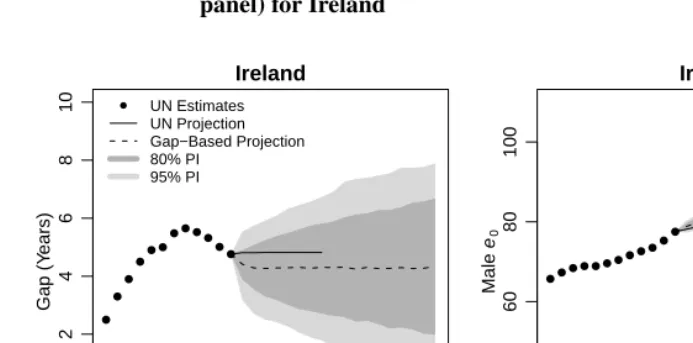
UN estimates of the gap in life expectancy between females and males in Ireland for the period 1950-2010 are displayed in the the left panel of Figure 4, along with the WPP 2008 projection, our median projection, and our 80% and 95% prediction intervals (PI). These same measures for male life expectancy at birth are presented in the right panel. The UN does not explicitly produce projections of the gap in life expectancy: we calculated both UN estimates and projections of the gap by subtracting estimates and projections of female life expectancy from estimates and projections of male life expectancy.

UN estimates show that Ireland experienced an increase in the gap between female and male life expectancy between the 1950-1955 and 1985-1990 quinquennia, from a gap of 2.5 years to a gap of 5.6 years. It then began a decline, reaching an estimated gap of 4.8 years in the 2005-2010 quinquennium. WPP 2008 projects the gap between female and male life expectancy to remain at 4.8 years for the entire period 2011-2050. Our model predicts similar stability in the gap, though it projects that gap to be 4.3 rather than 4.8 years between 2015 and 2050. We expect the gap to remain at 4.3 years in the 2095-2100 quinquennium with an 80% PI of [2.0, 6.7].

(18)

Figure 4: Estimates and projections of the gap in life expectancy between females and males (left panel) and of male life expectancy (right panel) for Ireland

0

2

4

6

8

10

Ireland

Gap (Y

ears)

1953 1963 1973 1983 1993 2003 2013 2023 2033 2043 2053 2063 2073 2083 2093

● _{UN Estimates} UN Projection Gap−Based Projection 80% PI

95% PI

● ●

● ●● ●

● ● ● ● ●

●

40

60

80

100

Ireland

Male

e0

1953 1963 1973 1983 1993 2003 2013 2023 2033 2043 2053 2063 2073 2083 2093 ●● ●

● ● ●● ● ● ●●

●

Notes: WPP 2008 estimates are shown as black circles; WPP 2008 projections to 2050 are shown as a solid black

line. The median projection using our gap-based model is shown as a dashed line, along with its 80% and 95% prediction intervals (PIs)

5.2 Guatemala

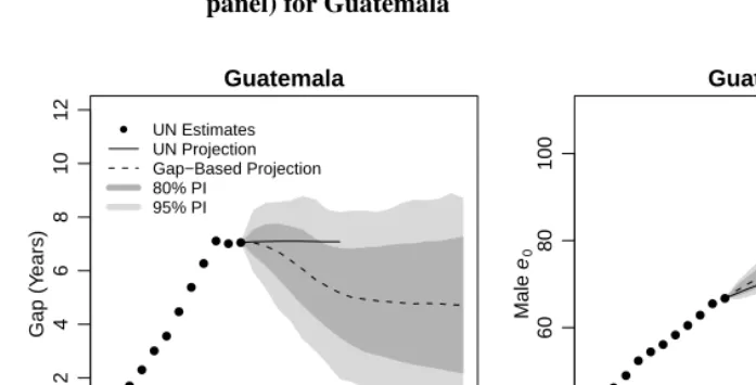
Guatemala has not yet experienced a narrowing of the gap between the life expectancy at birth of females and males, as can be seen in Figure 5. Indeed, the gap increased from just 0.5 years in 1950-1955 to 7.1 years in 1995-2000, and stagnated at 7.0 years through 2010. The UN projects that the gap will remain constant between 2010-2050 at a level of 7.1 years. However, our model suggests that after a brief rise to 7.1 years in the 2010-2015 quinquennium (80% PI [6.6, 7.5]), the gap will begin to decrease, dropping to 5.2 years (80% PI [3.5, 6.8]) in the 2045-2050 quinquennium, and to 4.7 years (80% PI [2.2, 7.3]) in the 2095-2100 quinquennium.

The uncertainty in the BHM projection ofe0for females in Guatemala is greater than

(19)

Figure 5: Estimates and projections of the gap in life expectancy between females and males (left panel) and of male life expectancy (right panel) for Guatemala

0 2 4 6 8 10 12 Guatemala Gap (Y ears)

1953 1963 1973 1983 1993 2003 2013 2023 2033 2043 2053 2063 2073 2083 2093

● _{UN Estimates} UN Projection Gap−Based Projection 80% PI 95% PI ● ● ● ● ● ● ● ● ● ● ● ● 40 60 80 100 Guatemala Male e0

1953 1963 1973 1983 1993 2003 2013 2023 2033 2043 2053 2063 2073 2083 2093 ●● ●● ●● ●● ●● ● ●

line. The median projection using our gap-based model is shown as a dashed line, along with its 80% and 95% PIs

The gap-based median projections of male life expectancy at birth are higher than the WPP 2008 projection. While WPP 2008 projects a life expectancy of 74.5 in 2045-2050, the gap-based median projection is 79.0 (80% PI [75.1, 82.4]).

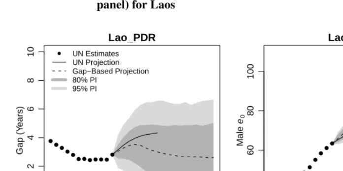
5.3 Laos

(20)

Figure 6: Estimates and projections of the gap in life expectancy between females and males (left panel) and of male life expectancy (right panel) for Laos

0

2

4

6

8

10

Lao_PDR

Gap (Y

ears)

1953 1963 1973 1983 1993 2003 2013 2023 2033 2043 2053 2063 2073 2083 2093

95% PI

●_● ●

●_● ● ● ● ● ● ●●

40

60

80

100

Lao_PDR

Male

e0

1953 1963 1973 1983 1993 2003 2013 2023 2033 2043 2053 2063 2073 2083 2093 ● ●● ●

●● ●●

● ●●

●

line. The median projection using our gap-based model is shown as a dashed line, along with its 80% and 95% PIs

Once again, our median projections of male life expectancy for Laos under the gap-based model are higher than the WPP 2008 projection, with WPP 2008 projecting a life expectancy of 73.6 years in 2045-2050, while the gap-based projection is 81.6 (80% PI [73.9, 89.4]). The prediction intervals for male life expectancy in Laos are much wider than for Guatemala or Ireland, which is consistent with the higher uncertainty involved in projecting these demographic quantities in Laos.

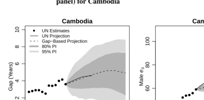
5.4 Cambodia

(21)

Figure 7: Estimates and projections of the gap in life expectancy between females and males (left panel) and of male life expectancy (right panel) for Cambodia

0

2

4

6

8

10

Cambodia

Gap (Y

ears)

1953 1963 1973 1983 1993 2003 2013 2023 2033 2043 2053 2063 2073 2083 2093

95% PI

● ●● ●●_● ● ● ●

● ● ●

40

60

80

100

Cambodia

Male

e0

1953 1963 1973 1983 1993 2003 2013 2023 2033 2043 2053 2063 2073 2083 2093 ●●

●● ●

● ●

●● ● ●

●

Notes: WPP 2008 estimates are shown as black circles; WPP 2008 projections to 2050 are shown as a black line.

The median projection using our gap-based model is shown as a dashed line, along with its 80% and 95% PIs.

In this case, the WPP 2008 projection for the gap and our model’s median projections agree quite well, even regarding the pace of the increase in the gap. In the 2045-2050 quinquennium, WPP 2008 projects a gap of 4.6 years, while our model’s median projec-tion is 4.7 years, with an 80% PI of [3.2, 6.3]. We project that this gap will rise to 5.2 years (80% PI [3.1, 7.1]) in the 2070-2075 quinquennium and remain at that level for about 15 years before beginning to drop. Our median projection for the 2095-2100 quinquennium is 4.9 years (80% PI [2.3, 7.3]). Because female life expectancy in Cambodia is relatively low (62.6 years in 2005-2010), our model projects a growth in the gap, following the trend of other countries. Thus, the case of Cambodia shows that our model can, and does, project increasing trajectories for the gap.

(22)

6. Discussion

We have described a methodology for joint probabilistic projection of female and male life expectancy. This methodology is built on previous work by Raftery et al. (2013) which uses a Bayesian hierarchical model framework to enhance the flexibility of the double-logistic function of gains in life expectancy used by the UN and produces projections of life expectancy for each sex independently. We start with probabilistic projections of life expectancy for females from the Bayesian hierarchical model. We then model the gap in life expectancy between females and males. Finally, we obtain corresponding projections of male life expectancy by combining these two quantities.

Because our goal is to project the gap in life expectancy between the sexes for all countries, our model must be based only on available data, be comparable across coun-tries, and account for possible shocks such as wars, as observed in the past. Thus we model the gap in the current period for a particular country simply as a function of the gap in the previous period and female life expectancy in the current period and in 1950– 1955 in that country, and at-distributed random perturbation based on the experience of all countries. Having observed that high-income countries that have reached high levels of female life expectancy have also experienced a narrowing in the gap between the sexes, we project that developing countries will follow the same trend.

We estimated all the parameters of our model based on life expectancy estimates re-ported in WPP 2008. We evaluated it using out-of-sample projections for the period 1995-2010, and compared our results to current UN methods as well as to probabilis-tic projections of the gap based on independent female and male projections of life ex-pectancy. We show that our model performs better than several independent projections of male and female life expectancy in terms of coverage, precision, and accuracy. The method is implemented in the freely available bayesLife and bayesDem R packages.

Despite its good performance, we recognize that our model is subject to several limi-tations, the first of which is our choice of covariates. Often, life expectancy is projected based on expectations about the impact of cause-specific mortality rates (Bongaarts 2009). Indeed, sex differences in mortality could be explained by many factors, including differ-ences in the distribution of social and biological protective and risk factors by sex, such as socioeconomic status, social relationships, health behaviors, and biological indicators of health (see Rogers et al. 2010 for a review of these factors). Also, it has been shown that the narrowing sex differences in mortality in high-income nations could be partly due to smoking patterns (Pampel 2005; Preston and Wang 2006; National Research Council 2011; Soneji and King 2011), and that differences in the pattern of the decline in the gap in various countries could be explained in part by the pattern of cigarette consumption (Staetsky 2009; Bobak 2003).

(23)

expectancy should be based on differences in expectations of improvements in cause-specific mortality rates for one sex relative to the other, or on smoking patterns, as in pre-vious studies in high-income countries (Pampel 2005; Preston and Wang 2006). However, doing so would require projecting many socioeconomic factors that affect a population’s health, while facing a lack of reliable data for even basic demographic quantities in many countries. While this is impossible for the moment, it is a potential source of improvement in the future. However, as Booth (2006) noted, making projections of socioeconomic fac-tors shifts the focus of the forecasting problem from the demographic variables to their determinants, while it may be harder to forecast the determinants, even given good data, than to directly forecast the variable (Keyfitz 1982).

Other statistical formulations of the model would be possible. Our goal is to project female and male life expectancy jointly, and so a structural vector autoregressive model could be used. However, in its standard linear form, such a model would not be able to incorporate the first increasing and then decreasing expected size of the gap given female life expectancy.

Also, we have used the Bayesian hierarchical model of Raftery et al. (2013) to project female life expectancy, while our model of the gap conditional on female life expectancy is frequentist. Using a Bayesian hierarchical model for female life expectancy had four main advantages. First, the patterns of change in female life expectancy varied markedly by country, and the hierarchical model was able to represent this. Second, the hierarchical model allowed the country-specific patterns to be estimated in a stable way by “borrow-ing strength” from the experience of other countries, effectively us“borrow-ing the data from other countries to construct a prior distribution. Third, the Bayesian approach allows relatively straightforward estimation using the Markov chain Monte Carlo simulation method. The hierarchical model could, in principle, be estimated in a frequentist manner by maximum likelihood, but this would be complicated as it would involve integrating over the country-specific double logistic curve parameters. These are effectively six-dimensional nonlinear random effects, so this would not be an easy task. Finally, the Bayesian approach allows the incorporation of external information via the prior distribution. This is particularly important for thezc_{parameters in equation (2) and the}_z_{parameter in equation (5), which} define the country-specific asymptotic levels of female life expectancy increase, and their world distribution. Because they refer largely to the future, they are not estimated very precisely by the data on the past, and so the external information on such levels in Oeppen and Vaupel (2002) was useful in specifying a reasonable range for these parameters; see Raftery et al. (2013). To balance these advantages, the Bayesian approach has the disad-vantage that it requires the specification of a prior distribution even when little external information is available.

(24)

ways that cannot be accomodated by a single probability model, and we did not use ex-ternal information in estimating the parameters. Thus, for modeling the gap, we used a frequentist approach; this does not require the specification of a prior distribution. One could view our frequentist gap model as approximating a Bayesian one, and the approx-imation is likely to be close because there is a substantial amount of data to estimate all the parameters. For further discussion of the choice between Bayesian and frequentist approaches in specific statistical problems, see Efron (2013).

To assess the full implications of our results for the future age- and sex-distribution of the population would require us to generate full probabilistic population projections based on our joint projections of female and male life expectancy. This could be done using the method of Raftery et al. (2012), for example. Broadly, given that our projections of the gap between female and male life expectancy are lower than the WPP 2008 projections for most countries, this means that we generally project males to live longer than does the WPP 2008. We expect greater male longevity to result in larger numbers of older individuals, and a more even sex balance amongst the old. More generally, our results suggest that the present methodology may yield more accurate forecasts of female and male life expectancies, and their uncertainty, for most countries in the world.

7. Acknowledgements

(25)

References

Alkema, L., Raftery, A.E., Gerland, P., Clark, S.J., Pelletier, F., Buettner, T., and Heilig, G.K. (2011). Probabilistic Projections of the Total Fertility Rate for All Countries.

Demography48(3): 815–839. doi:10.1007/s13524-011-0040-5.

Austad, S.N. (2011). Sex Differences in Longevity and Aging. In: Masoro, E.J. and Austad, S.N. (eds.). Handbook of the Biology of Aging (Seventh Edition). Academic Press: 479–495. doi:10.1016/B978-0-12-378638-8.00023-3.

Bassil, N. and Morley, J.E. (2010). Late-Life Onset Hypogonadism: A Review. Clinics

in Geriatric Medicine26(2): 197–222. doi:10.1016/j.cger.2010.02.003.

Bobak, M. (2003). Relative and absolute gender gap in all-cause mortality in Europe and the contribution of smoking. European Journal of Epidemiology18(1): 15–18.

doi:10.1023/A:1022556718939.

Bongaarts, J. (2009). Trends in senescent life expectancy. Population Studies 63(3): 203–213.doi:10.1080/00324720903165456.

Booth, H. (2006). Demographic forecasting: 1980 to 2005 in review. International

Journal of Forecasting22(3): 547–581. doi:10.1016/j.ijforecast.2006.04.001.

Cairns, A.J.G., Blake, D., Dowd, K., Coughlan, G.D., Epstein, D., and Khalaf-Allah, M. (2011). Mortality density forecasts: An analysis of six stochas-tic mortality models. Insurance: Mathematics and Economics 48(3): 355–367.

doi:10.1016/j.insmatheco.2010.12.005.

Conti, S., Farchi, G., Masocco, M., Minelli, G., Toccaceli, V., and Vichi, M. (2003). Gender differentials in life expectancy in italy. European Journal of Epidemiology

18(2): 107–112. doi:10.1023/A:1023029618044.

Efron, B. (2013). Bayes’ Theorem in the 21st Century. Science340(6137): 1177–1178.

doi:10.1126/science.1236536.

Elo, I.T. and Drevenstedt, G.L. (2005). Cause-specific contributions to sex differences in adult mortality among whites and African Americans between 1960 and 1995.

Demo-graphic Research13(19): 485–520.doi:10.4054/DemRes.2005.13.19.

Emslie, C. and Hunt, K. (2008). The weaker sex? Exploring lay understandings of gender differences in life expectancy: A qualitative study. Social Science & Medicine67(5): 808 – 816.doi:10.1016/j.socscimed.2008.05.009.

(26)

627.doi:10.1016/j.rmed.2007.12.009.

Girosi, F. and King, G. (2008). Demographic Forecasting. Princeton, NJ: Princeton University Press.

Gjonça, A., Tomassini, C., and Vaupel, J.W. (1999). Male-female differences in mortality in the developed world. Rostock, Germany: Max Planck Institute for Demographic Research: 11–111. (Working Paper No. 009).

Glei, D.A. and Horiuchi, S. (2007). The narrowing sex differential in life expectancy in high-income populations: Effects of differences in the age pattern of mortality.

Popu-lation Studies61(2): 141–159. doi:10.1080/00324720701331433.

Gómez-Redondo, R. and Boe, C. (2005). Decomposition analysis of Spanish life ex-pectancy at birth: Evolution and changes in the components by sex and age.

Haberman, S. and Renshaw, A. (2008). Mortality, longevity and experiments with the Lee-Carter model. Lifetime Data Analysis14(3): 286–315.

doi:10.1007/s10985-008-9084-2.

Heilig, G.K., Buettner, T., Li, N., Gerland, P., Pelletier, F., Alkema, L., Chunn, J., Ševˇcíková, H., and Raftery, A.E. (2010). A probabilistic version of the United Na-tions World Population Prospects: Methodological improvements by using Bayesian

fertility and mortality projections. Lisbon: Joint Eurostat/UNECE Work Session on

Demographic Projections.

Hyndman, R.J., Booth, H., and Yasmeen, F. (2013). Coherent Mortality Forecasting: The Product-Ratio Method With Functional Time Series Models. Demography50(1): 261–283.doi:10.1007/s13524-012-0145-5.

Hyndman, R.J. and Shahid Ullah, M. (2007). Robust forecasting of mortality and fertility rates: A functional data approach. Computational Statistics & Data Analysis51(10): 4942–4956.doi:10.1016/j.csda.2006.07.028.

Keyfitz, N. (1982). Can Knowledge Improve Forecasts? Population and Development

Review8(4): 729–751.

Kołodziej, H., Łopusza´nska, M., and Jankowska, E. (2008). Decrease in sex difference in premature mortality during system transformation in poland. Journal of Biosocial

Science40: 297–312.doi:10.1017/S0021932007002453.

(27)

Lee, R.D. and Carter, L.R. (1992). Modeling and Forecasting U.S. Mor-tality. Journal of the American Statistical Association 87(419): 659–671.

doi:10.1080/01621459.1992.10475265.

Li, N. and Lee, R.D. (2005). Coherent mortality forecasts for a group of popu-lations: An extension of the Lee-Carter method. Demography 42(3): 575–594.

doi:10.1353/dem.2005.0021.

Lord, C., Engert, V., Lupien, S.J., and Pruessner, J.C. (2010). Effect of sex and estrogen therapy on the aging brain: a voxel-based morphometry study.Menopause17(4): 846–

851. doi:10.1097/gme.0b013e3181e06b83.

Maklakov, A.A. (2008). Sex difference in life span affected by female birth

rate in modern humans. Evolution and Human Behavior 29(6): 444–449.

doi:10.1016/j.evolhumbehav.2008.08.002.

Meslé, F. (2004). Écart d’espérance de vie entre les sexes : les raisons du recul de l’avantage féminin. Revue d’Épidémiologie et de Santé Publique 52(4): 333–352.

doi:10.1016/S0398-7620(04)99063-3.

Müller, H.G., Chiou, J.M., Carey, J.R., and Wang, J.L. (2002). Fertility and Life Span: Late Children Enhance Female Longevity. The Journals of

Geron-tology Series A: Biological Sciences and Medical Sciences 57(5): B202–B206.

doi:10.1093/gerona/57.5.B202.

National Research Council (2011). Explaining Divergent Levels of Longevity in

High-Income Countries. Washington, D.C.: National Academies Press.

Neumayer, E. and Plümper, T. (2007). The Gendered Nature of Natural Disasters: The Impact of Catastrophic Events on the Gender Gap in Life Expectancy, 1981–2002.

An-nals of the Association of American Geographers97(3): 551–566.

doi:10.1111/j.1467-8306.2007.00563.x.

Oeppen, J. and Vaupel, J.W. (2002). Broken Limits to Life Expectancy. Science

296(5570): 1029–1031.doi:10.1126/science.1069675.

Owens, I.P.F. (2002). Sex Differences in Mortality Rate.Science297(5589): 2008–2009.

doi:10.1126/science.1076813.

Pampel, F.C. (2005). Forecasting sex differences in mortality in high income na-tions: The contribution of smoking. Demographic Research 13(18): 455–484.

doi:10.4054/DemRes.2005.13.18.

(28)

754.doi:10.1017/S0020818306060231.

Preston, S.H. and Wang, H. (2006). Sex mortality differences in The United States: The role of cohort smoking patterns. Demography 43(4): 631–646.

doi:10.1353/dem.2006.0037.

Raftery, A.E., Chunn, J.L., Gerland, P., and Ševˇcíková, H. (2013). Bayesian Probabilis-tic Projections of Life Expectancy for All Countries. Demography50(3): 777–801.

doi:10.1007/s13524-012-0193-x.

Raftery, A.E., Li, N., Ševˇcíková, H., Gerland, P., and Heilig, G.K. (2012). Bayesian prob-abilistic population projections for all countries.Proceedings of the National Academy

of Sciences109(35): 13915–13921.doi:10.1073/pnas.1211452109.

Rogers, R.G., Everett, B.G., Onge, J.M.S., and Krueger, P.M. (2010). Social, behavioral, and biological factors, and sex differences in mortality. Demography47(3): 555–578.

doi:10.1353/dem.0.0119.

Ševˇcíková, H. (2013). bayesDem: Graphical User Interface for bayesTFR, bayesLife and bayesPop. [electronic resource]. R package version 2.3-2.

Ševˇcíková, H. and Gerland, P. (2014). wpp2008: World Population Prospects 2008. [elec-tronic resource]. R package version 1.0-1.

Ševˇcíková, H. and Raftery, A.E. (2014). bayesLife: Bayesian Projection of Life Ex-pectancy. [electronic resource]. R package version 2.1-0.

Shang, H.L., Booth, H., and Hyndman, R.J. (2011). Point and interval forecasts of mor-tality rates and life expectancy: A comparison of ten principal component methods.

Demographic Research25(5): 173–214.doi:10.4054/DemRes.2011.25.5.

Soliani, L. and Lucchett, E. (2006). Genetic factors in mortality. In: Caselli, G., Vallin, J., and Wunsch, G.J. (eds.).Demography: Analysis and Synthesis. Amsterdam: Elsevier: 117–128.

Soneji, S. and King, G. (2011). The future of death in America.Demographic Research

25(1): 1–38.doi:10.4054/DemRes.2011.25.1.

Staetsky, L. (2009). Diverging trends in female old-age mortality: A reappraisal.

Staetsky, L. and Hinde, A. (2009). Unusually small sex differentials in mortality of Israeli Jews: What does the structure of causes of death tell us? Demographic Research

20(11): 209–252.doi:10.4054/DemRes.2009.20.11.

(29)

version 0.3.

Taylor, J. and Verbyla, A. (2004). Joint modelling of location and scale parameters of the t distribution. Statistical Modelling4(2): 91–112. doi:10.1191/1471082X04st068oa.

Trovato, F. and Heyen, N.B. (2006). A varied pattern of change of the sex differ-ential in survival in the g7 countries. Journal of Biosocial Science 38: 391–401.

doi:10.1017/S0021932005007212.

Trovato, F. and Lalu, N.M. (1996). Narrowing sex differentials in life expectancy in the industrialized world: early 1970’s to early 1990’s. Social Biology43: 20–37.

Trovato, F. and Lalu, N.M. (1998). Contribution of cause-specific mortality to changing sex differences in life expectancy: seven nations case study.Biodemography and Social

Biology45(1–2): 1–20.doi:10.1080/19485565.1998.9988961.

Trovato, F. and Lalu, N.M. (2007). From divergence to convergence: The sex differen-tial in life expectancy in Canada, 1971–2000. Canadian Review of Sociology/Revue

canadienne de sociologie44: 101–122.

Trovato, F. and Odynak, D. (2011). Sex differences in life expectancy in Canada: Im-migrant and native-born populations. Journal of Biosocial Science 43: 353–367.

doi:10.1017/S0021932011000010.

United Nations (2006). World Mortality Report 2005. New York, NY: United Nations.

United Nations (2009).World Population Prospects: The 2008 Revision. New York, NY: United Nations.

United Nations (2011).World Population Prospects: The 2010 Revision. New York, NY: United Nations.

Vallin, J. (2006). Mortality, sex, and gender. In: Caselli, G., Vallin, J., and Wunsch, G.J. (eds.).Demography: Analysis and Synthesis, Volume II. Academic Press: 177–194.

(30)