Volume 19 - Article 35 | Pages 1323–1350

(1)

in the population sciences published by the Max Planck Institute for Demographic Research Konrad-Zuse Str. 1, D-18057 Rostock·GERMANY www.demographic-research.org

DEMOGRAPHIC RESEARCH

VOLUME 19, ARTICLE 35, PAGES 1323-1350

PUBLISHED 25 JULY 2008

http://www.demographic-research.org/Volumes/Vol19/35/ DOI: 10.4054/DemRes.2008.19.35

Research Article

An integrated approach to cause-of-death

analysis: cause-deleted life tables and

decompositions of life expectancy

Hiram Beltrán-Sánchez

Samuel H. Preston

Vladimir Canudas-Romo

c

°2008 Beltrán-Sánchez, Preston, and Canudas-Romo.

(2)

1 Introduction 1324

2 Background 1324

3 Decomposition approaches 1326

4 Relation between the decomposition approach and cause-deleted

life tables 1327

5 Application to recent mortality change in the United States 1329

5.1 Decomposition of changes by causes of death 1329

5.1.1 Results 1330

5.2 Cause-deleted life tables and changes therein 1331

6 Summary 1340

References 1342

Appendix 1 1345

Appendix 2 1347

(3)

An integrated approach to cause-of-death analysis: cause-deleted life

tables and decompositions of life expectancy

Hiram Beltrán-Sánchez1

Samuel H. Preston2

Vladimir Canudas-Romo3

Abstract

This article integrates two methods that analyze the implications of various causes of death for life expectancy. One of the methods attributes changes in life expectancy to various causes of death; the other method examines the effect of removing deaths from a particular cause on life expectancy. This integration is accomplished by new formulas that make clearer the interactions among causes of death in determining life expectancy. We apply our approach to changes in life expectancy in the United States between 1970 and 2000. We demonstrate, and explain analytically, the paradox that cancer is responsible for more years of life lost in 2000 than in 1970 despite the fact that declines in cancer mortality contributed to advances in life expectancy between 1970 and 2000.

1_{Population Studies Center, University of Pennsylvania, 3718 Locust Walk, Philadelphia, PA 19104-6298.} E-mail: [email protected].

2_{Population Studies Center, University of Pennsylvania. E-mail: [email protected].}

(4)

1. Introduction

When measured for a particular period, life expectancy at birth is a summary measure of the mortality conditions of that period. Estimating the role of causes of death in determining the level of life expectancy, and changes therein, is an active area of de-mographic research. Two broad research approaches have been employed: analyzing the life-shortening effect of causes of death if a cause were eliminated; and attributing changes or differences in life expectancy to various causes of death. The first approach is focused on a single population and has led to the development of single decrement (often, “cause-deleted”) life tables. The second approach is comparative and has lead to the de-velopment of decomposition methods that assign responsibility for mortality variation to particular causes of death.

The approaches are related but the relations have not been demonstrated. In this paper, we develop new expressions for decomposition methods and show that they are related in a straightforward way to expressions characterizing cause-deleted tables. We apply the analytic framework to data for the United States between 1970 and 2000.

2. Background

Although demographers have long used life tables to analyze mortality from all causes combined, the development of life tables that highlight the role of various causes of death is more recent (Brownlee 1919; Fisher, Vigfusson, and Dickson 1922; Pearl 1922; Gre-ville 1948; Jordan 1952; Chiang 1968; Spiegelman 1968, Preston, Keyfitz, and Schoen 1972). The first official decennial life table by cause of death for the United States was published in the late 1960’s (United States. Dept. of Health, Education, and Welfare 1968).

One of the most important products of such life tables is the estimated gain in life ex-pectancy at birth if a particular cause of death were eliminated, i.e., if the death rate from that cause were arbitrarily set to zero while death rates from all other causes remained

the same. To recapitulate the mathematics of such a calculation, suppose that there aren

mutually exclusive and exhaustive causes of death operating in a population at timet. The

probability of surviving from birth to ageaat timetif the only cause of death operating

were causeiis

pi(a, t) =e

−Ra

0

µi(s,t) ds

,

whereµi(s, t)is the death rate from causeiin the age intervalstos+ds. In the life table

(5)

p(a, t) =e−

a R 0

µ(s,t) ds

, where µ(s, t) =

n X

i=1

µi(s, t).

For simplicity, letp(a, t) =p(a).

If we assume thencauses of death to be independent,p(a) =p1(a)·p2(a)·. . .·pn(a).

Letp−i(a) = _pip(₍a_a)₎ be the probability of surviving from all causes except causeiat age

a. Given the force of mortality,µ(s), life expectancy at birth is computed as

e(0) =

ω Z

0 e−

a R 0

µ(s) ds

da=

ω Z

0

p(a) da.

If there arenmutually exclusive and exhaustive causes of death operating in a population

then life expectancy is computed as

e(0) =

ω Z

0

p1(a)p2(a). . . pn(a) da.

LetDi(0)be the years of life gained at birth if cause of deathiwere eliminated. Then

Di(0)is computed as:

Di(0) = ω Z

0

p−i(a) da− ω Z

0

p−i(a)pi(a) da. (1)

(6)

3. Decomposition approaches

In the early 1980’s, a technique to decompose changes in life expectancy by age and cause of death was independently developed by Arriaga (1982; 1984), Andreev (1982), Pollard (1982), and Pressat (1985). These versions are mathematically equivalent (Pollard 1988), although their implementation via various discrete approximations can give rise to different results, as shown below. Later developments applied decomposition methods to other demographic measures and introduced dynamic elements (Andreev et al. 2002; Vaupel and Canudas-Romo 2002; Vaupel and Canudas-Romo 2003).

The initial target and main focus of decomposition techniques was not on causes of death but on age. Decompositions of trends or differences in mortality by age preceded cause-decompositions and the latter decompositions were designed along the lines of the former. Had the initial target been cause-decompositions, a more straightforward set of expressions was available, which is now developed.

As shown above, if there are nmutually exclusive and exhaustive causes of death

operating in a population thenp(a) = p1(a)·p2(a)·. . .·pn(a). If we assume that the

force of mortality (µ(a)) is differentiable with respect to time, then the change in the

probability of surviving from birth to ageawith respect to time can be written in the

following form:

˙

p(a) =

n X

i=1

˙

pi(a)p−i(a),

where a dot over a term represents the derivative with respect to time. Thus, the

continu-ous change in life expectancy at birth is given by4

˙

e(0) =

n X

i=1

ω Z

0

˙

pi(a)p−i(a) da. (2)

Equation (2) is a straightforward expression for decomposing variation in life ex-pectancy into various causes of death. It shows clearly that the contribution of each cause of death to the change in life expectancy is driven by the changes in cause specific

sur-vivorship (causei) weighted by the cumulative probability of surviving from the

remain-ing causes (cause−i). The integral in equation (2) can be subdivided into age-groups to

account for the age-contribution to the change in life expectancy. Thus, equation (2) can

return both cause- and age-contribution to the change ine(0). Equation (2) is the basis of

the connection between decomposition methods and cause-deleted life tables, as shown below.

(7)

For discrete time intervals, lete(0)ande∗₍₀₎_{represent the life expectancy at birth at} times 1 and 2, respectively. Then (see Appendix 1 in Beltrán-Sánchez and Preston (2007) for more details):

e∗(0)−e(0)∼=

n X

i=1

∞

Z

0

(p∗i −pi) (

p−i+p∗−i

2 ) da.

In discrete age intervals the above formula is equivalent to

e∗₍₀₎₋_e_{(0) =}

n X

i=1

ω X

x=0,5

(nL∗x,i−nLx,i) (

nL∗x,−i+nLx,−i

2n ),

wherenLx,i,nLx,−i,nL∗x,i,nL∗x,−irepresent the person-years lived between agesxand

x+nat times 1 and 2 in the life tables for causeiand cause−i, respectively, using a life

table radix of 1 (see Appendix 3 for more details).

Appendix Table A1 compares results from implementing our approach to cause-of-death decompositions to those of Pollard and Arriaga. Differences are found to be minute between our approach and Pollard’s. Relative to the other two approaches, Arriaga’s approach can underestimate the importance of major causes of death heavily concentrated at older ages.

4. Relation between the decomposition approach and cause-deleted

life tables

As shown in equation (1), the years of life gained at birth at timetif cause of deathiis

eliminated is computed as:

Di(0) = ω Z

0

p−i(a) da− ω Z

0

p−i(a)pi(a) da.

Thus, the change inDi(0)with respect to time is given by

˙

Di(0) = ω Z

0

˙

p−i(a)qi(a) da− ω Z

0

˙

pi(a)p−i(a) da, (3)

whereqi(a) = 1−pi(a)and a dot over a term represents the derivative with respect to

(8)

For discrete time intervals, letDi(0)andD∗i(0)represent the gain in life expectancy

at birth at times 1 and 2, respectively, by eliminating cause of deathi. Then, equation (3)

can be written as (see Appendix 2 for more details):

Di∗(0)−Di(0) =

∞

Z

0

(p∗−i−p−i) (qi+q

∗

i

2 ) da− ∞

Z

0

(p∗i −pi) (

p−i+p∗−i

2 ) da,

whereqi= 1−pi.

In discrete age intervals the above formula is equivalent to

D∗

i(0)−Di(0) = ω X

x=0,5

(nL∗x,−i−nLx,−i) (1−

nLx,i+nL∗x,i

2n )

−

ω X

x=0,5

nLx,−i+nL∗x,−i

2n ).

Thus, the change in the number of years of life lost to a particular cause of death is a function of two terms. The second term in equation (3) is the change in survival

from causeiweighted by the cumulative probability of surviving from cause−i. From

equation (2), it is precisely the change in life expectancy at birth attributable to changes in

cause of deathi. Thus, thechangein the amount of life expectancy sacrificed to causeiin

cause-deleted life tables is closely connected to thechangein life expectancy attributable

to causeiin decomposition formulas. In fact, the two would be exactly the same if death

rates from other causes were constant, becausep˙−i(a)in the first term would then be zero.

In other words, apositivecontribution by a cause of death to changes in life expectancy

would exactly equal thereductionin years of life lost to that cause (hence the minus sign

on the second term of equation (3)). In general, the first term in equation (3) shows the

change in survival from cause−iweighted by the cumulative probability of dying from

causei. It would be large in magnitude only if causeiis an important cause of deathand

changes in cause−iare large.

(9)

time 1. Clearly, changes in its life-shortening effects depend on changes in mortality from other causes, a dependence that is made explicit in equation (3).

5. Application to recent mortality change in the United States

5.1 Decomposition of changes by causes of death

After several decades of slow improvement in mortality, the United States experienced substantial advances in longevity between 1970 and 2000. These are widely believed to reflect primarily reductions in death rates from cardiovascular diseases, facilitated by medical advances such as cardiovascular bypass surgery and expanded use of blood pres-sure reduction drugs, statins, and beta blockers, as well as by reductions in cigarette smo-king (Cutler 2004; Ergin et al. 2004; Ford et al. 2007).

Mortality data for 1970 are drawn from the publicly available multiple cause of death file, 1968-1973, obtained through the Inter-university Consortium for Political and Social Research (National Center for Health Statistics (NCHS) 2001). For the year 2000, we use the multiple cause of death public use file published by the National Center for Health Statistics (2002). The midyear population figures in 1970 and 2000 are drawn from the

Census Bureau (U.S. Bureau of the Census 1971; U.S. Bureau of the Census 2005).5

For blacks in 1970 we use the size of the African-American population reconstructed by

Preston et al. (1998).6 _{The terminal age category in our application is age 100+.}7 _We

focus on the eleven leading causes of death in the U.S. for the year 2000 and construct

comparable categories in 1970.8 _{We use the following groups: heart disease;}

cerebrovas-cular diseases; malignant neoplasms; chronic lower respiratory diseases; violence (ac-cidents (unintentional injuries), intentional self-harm (suicide), and assault (homicide)); diabetes; influenza-pneumonia; nephritis (nephritis, nephrotic syndrome and nephrosis); septicemia; liver cirrhosis (chronic liver disease and cirrhosis); and hypertension (essen-tial (primary) hypertension and hypertensive renal disease). Comparable codes for 1970 were derived from Centers for Disease Control and Prevention (CDC) (2001).

5_{For the year 2000 we use the electronically available monthly postcensal estimation of the resident} popu-lation.

6_{We use Preston et al. (1998) estimates for ages 0-84, and census estimates for ages 85-99 (U.S. Bureau of} the Census 1971).

7_{The centenarian population in 1970 was improperly counted (Siegel 1974). Thus, we use the preferred} estimates of centenarians by race and sex from Siegel and Passel (1976).

(10)

5.1.1 Results

We estimate life expectancy at birth for the total U.S. population in 1970 to be 70.70 years (slightly lower than the value of 70.9 estimated by the NCHS (1974)) and 76.96 years for the year 2000 (slightly higher than the value of 76.9 estimated by Arias (2002)). Thus, life expectancy at birth is estimated to have increased by about 6.26 years between 1970 and 2000 for the total population of the U.S. Comparable figures by race and sex are shown in Table 1.

Table 1: Change in life expectancy at birth for the U. S. population by race and sex between 1970 and 2000

Year Total Population White Population Black Population All Males Females All Males Females All Males Females

2000 76.96 74.24 79.56 77.44 74.79 79.99 71.74 68.15 75.06 1970 70.70 66.97 74.62 71.58 67.88 75.46 64.78 61.16 68.66

Difference 6.26 7.27 4.94 5.86 6.91 4.53 6.96 6.99 6.40

Source:Multiple cause of death file (1968-1973), multiple cause of death 2000, and census bureau estimates.

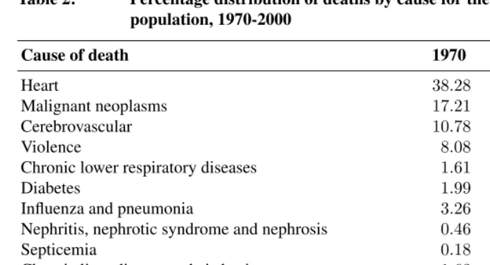
The eleven causes of death selected in this study account for the majority of the deaths in both time periods. In 1970, about 84% of the total deaths were attributed to one of those eleven causes for the total population, and in 2000, the percentage slightly decreased to about 80% (Table 2). Cardiovascular diseases (heart and cerebrovascular) and malignant neoplasms are responsible for 66% of deaths in 1970 and 59% in 2000.

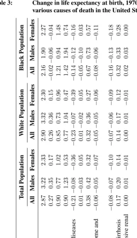
Our estimates of the contribution of each cause of death to the change in life ex-pectancy at birth by race and sex between 1970 and 2000 are shown in Table 3 and

Figure 1.9 _{Heart disease contributed the majority of the increase in life expectancy at}

birth during the 30-year period for all groups except black males, for whom large

(11)

Table 2: Percentage distribution of deaths by cause for the total U. S. population, 1970-2000

Cause of death 1970 2000

Heart 38.28 29.58

Malignant neoplasms 17.21 23.00

Cerebrovascular 10.78 6.98

Violence 8.08 5.29

Chronic lower respiratory diseases 1.61 5.07

Diabetes 1.99 2.88

Influenza and pneumonia 3.26 2.72

Nephritis, nephrotic syndrome and nephrosis 0.46 1.55

Septicemia 0.18 1.30

Chronic liver disease and cirrhosis 1.63 1.11

Hypertension and hypertensive renal disease 0.43 0.75

All other 16.07 19.79

Sum 100.00 100.00

Source:see Table 1.

clines in death rates from violence contributed 1.94 years of life to the total gain of 6.99 years. This exceptionally large decline in violent mortality resulted in a larger gain in life expectancy for black males than for any other race/sex group during the period. Can-cers made a positive contribution to life expectancy gains for the total population and for whites but not for blacks. Diabetes also shows a negative contribution but among males only.

5.2 Cause-deleted life tables and changes therein

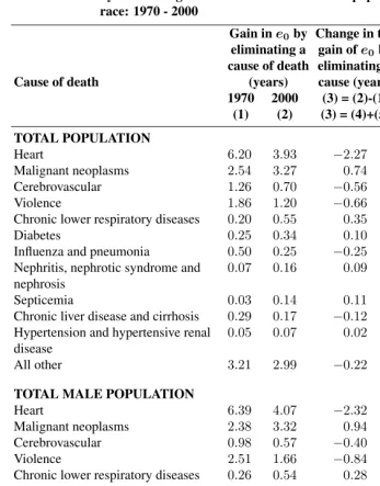
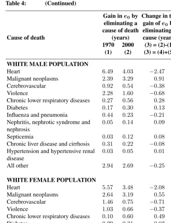
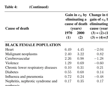
Table 4 and Figure 2 show the estimated gain in life expectancy from eliminating a partic-ular cause of death in 1970 and 2000, using formula (1). Table 4 also shows, in column 3,

the change in this quantity between 1970 and 2000. These values correspond to “D˙i(0)”

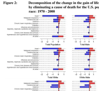
in formula (3). Column 4 (red color in Figure 2) and column 5 (blue color in Figure 2) of the table present the two elements on the right-hand side of formula (3). Column 5 is simply the change in life expectancy attributable to a particular cause of death (i.e., the result of our decomposition of mortality change by cause) while Column 4 represents the

(12)

Table 3: Change in life expectancy at birth, 1970-2000, attributable to various causes of death in the United States (in years)

(13)

death during the period. Without such interference from other causes, columns 3 and 5 would be identical.

Figure 1: Change in life expectancy at birth attributable to various causes of death in the United States (in years): 1970 - 2000

Source:Table 3

(14)

responsible for about 2.4 times the loss of life years of neoplasms. In 2000, the ratio was only 1.2.

Even though the death rate from neoplasms was slowly declining between 1970 and 2000, more years of life were actually sacrificed to neoplasms in 2000 than in 1970. The average number of years of life lost to neoplasms grew by 0.74 for the population as a whole, by far the greatest increase for any cause. This value, shown in column 3, is the results of a contribution of +1.00 years from the “other cause change” term in column 4, partially offset by the -0.27 year term reflecting the decline in death rates from neoplasms themselves. In other words, the sole reason why more years of life are sacrificed to neoplasms in 2000 than in 1970 is the decline in death rates from other causes of death, most notably heart disease. If cancer death rates had not changed, cancer would have been responsible for the loss of 1.00 additional year of life in 2000. Because of the

decline in causes of deathother thancancer, those who died from cancer in 2000 would

otherwise have lived longer, on average, than those who died from cancer in 1970. As a result, cancer caused a greater loss of life in 2000 than in 1970 even though its death rates declined over this period. This result underscores the importance of interactions among diseases in determining longevity. The key interaction is made explicit in equation (3).

While extreme, the result pertaining to cancer is not unusual. In fact, the values in

column 4 are positive foreverycause of death for each of the race/sex groups. Declines

(15)

Table 4: Decomposition of the change in the gain of life expectancy at birth by eliminating a cause of death for the U. S. population by sex and race: 1970 - 2000

Gain ine0by Change in the

eliminating a gain ofe0by Equation (3) cause of death eliminating a First Second

Cause of death (years) cause (years) Term∗ _Term∗∗

1970 2000 (3) = (2)-(1) (4) (5) (1) (2) (3) = (4)+(5)

TOTAL POPULATION

Heart 6.20 3.93 −2.27 0.60 −2.87

Malignant neoplasms 2.54 3.27 0.74 1.00 −0.27

Cerebrovascular 1.26 0.70 −0.56 0.34 −0.90

Violence 1.86 1.20 −0.66 0.24 −0.90

Chronic lower respiratory diseases 0.20 0.55 0.35 0.15 0.21

Diabetes 0.25 0.34 0.10 0.11 −0.01

Influenza and pneumonia 0.50 0.25 −0.25 0.13 −0.38

Nephritis, nephrotic syndrome and nephrosis

0.07 0.16 0.09 0.04 0.06

Septicemia 0.03 0.14 0.11 0.02 0.08

Chronic liver disease and cirrhosis 0.29 0.17 −0.12 0.05 −0.17

Hypertension and hypertensive renal disease

0.05 0.07 0.02 0.02 0.00

All other 3.21 2.99 −0.22 0.88 −1.10

TOTAL MALE POPULATION

Heart 6.39 4.07 −2.32 0.91 −3.22

Violence 2.51 1.66 −0.84 0.39 −1.23

Diabetes 0.18 0.32 0.14 0.11 0.03

0.07 0.16 0.09 0.05 0.05

Septicemia 0.04 0.13 0.09 0.03 0.07

(16)

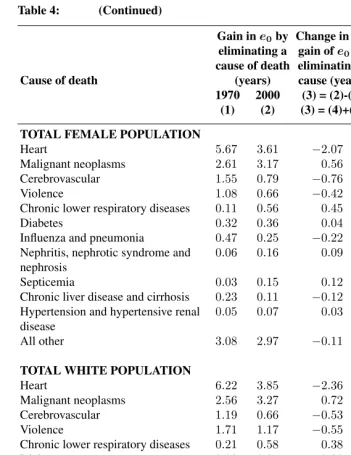
Table 4: (Continued)

1970 2000 (3) = (2)-(1) (4) (5) (1) (2) (3) = (4)+(5)

TOTAL FEMALE POPULATION

Heart 5.67 3.61 −2.07 0.27 −2.33

Violence 1.08 0.66 −0.42 0.11 −0.53

Diabetes 0.32 0.36 0.04 0.09 −0.05

0.06 0.16 0.09 0.03 0.07

Septicemia 0.03 0.15 0.12 0.02 0.10

0.05 0.07 0.03 0.02 0.01

All other 3.08 2.97 −0.11 0.77 −0.88

TOTAL WHITE POPULATION

Heart 6.22 3.85 −2.36 0.53 −2.90

Violence 1.71 1.17 −0.55 0.22 −0.77

Diabetes 0.23 0.31 0.08 0.10 −0.01

0.05 0.14 0.08 0.03 0.05

Septicemia 0.03 0.12 0.10 0.02 0.07

0.04 0.05 0.02 0.02 0.00

(17)

1970 2000 (3) = (2)-(1) (4) (5) (1) (2) (3) = (4)+(5)

WHITE MALE POPULATION

Heart 6.49 4.03 −2.47 0.86 −3.32

Violence 2.28 1.60 −0.68 0.36 −1.04

Diabetes 0.17 0.30 0.13 0.10 0.02

0.05 0.14 0.09 0.04 0.05

Septicemia 0.03 0.12 0.08 0.03 0.06

0.03 0.05 0.01 0.02 −0.01

All other 2.94 2.69 −0.25 0.89 −1.14

WHITE FEMALE POPULATION

Heart 5.57 3.48 −2.08 0.22 −2.30

Violence 1.03 0.66 −0.37 0.10 −0.47

Diabetes 0.29 0.31 0.03 0.08 −0.05

0.05 0.13 0.08 0.02 0.06

Septicemia 0.03 0.13 0.10 0.02 0.09

0.04 0.06 0.02 0.01 0.01

(18)

1970 2000 (3) = (2)-(1) (4) (5) (1) (2) (3) = (4)+(5)

TOTAL BLACK POPULATION

Heart 6.02 4.42 −1.60 0.56 −2.16

Malignant neoplasms 2.42 3.44 1.03 1.01 0.02

Violence 2.60 1.49 −1.12 0.31 −1.42

Diabetes 0.37 0.58 0.21 0.16 0.05

0.16 0.32 0.15 0.07 0.08

Septicemia 0.06 0.27 0.21 0.05 0.16

0.14 0.17 0.03 0.05 −0.02

All other 4.84 4.07 −0.77 0.84 −1.61

BLACK MALE POPULATION

Heart 5.40 4.17 −1.23 0.67 −1.90

Violence 3.72 2.20 −1.51 0.43 −1.94

Diabetes 0.23 0.45 0.22 0.12 0.10

0.15 0.28 0.13 0.07 0.06

Septicemia 0.06 0.24 0.18 0.04 0.13

0.13 0.14 0.01 0.05 −0.03

(19)

1970 2000 (3) = (2)-(1) (4) (5) (1) (2) (3) = (4)+(5)

BLACK FEMALE POPULATION

Heart 6.49 4.45 −2.04 0.23 −2.27

Violence 1.29 0.69 −0.60 0.14 −0.74

Diabetes 0.55 0.68 0.14 0.17 −0.03

0.17 0.35 0.17 0.07 0.11

Septicemia 0.07 0.30 0.23 0.04 0.18

0.15 0.19 0.04 0.04 0.00

All other 4.71 3.91 −0.80 0.72 −1.52

∗_{Effect of changes in other causes of death on years of life lost to the cause.} ∗∗_{Effect of changes in the cause itself on years of life lost.}

(20)

Figure 2: Decomposition of the change in the gain of life expectancy at birth by eliminating a cause of death for the U.S. population by sex and race: 1970 - 2000

∗_{Effect of changes in other causes of death on years of life lost to the cause.} ∗∗_{Effect of changes in the cause itself on years of life lost.}

Source:Table 4

6. Summary

(21)

these two types of analyses are closely related to one another. In particular, the change in the years of life lost to a particular disease is shown to be equal to the amount of change attributable to that disease in a cause-decomposition, plus a simple additional term that reflects movements in other causes of death. The public health significance of a disease is thus shown to be an outcome of a struggle among causes of death. If one cause declines more rapidly than others, in a manner made explicit in equation (3), that cause will be responsible for fewer years of life lost at the end of the period. Heart disease won that struggle over the period investigated, whereas the decline in cancer death rates was not sufficient to avert its becoming responsible for a greater loss of life at the end of the period than at the beginning.

(22)

References

Andreev, E. (1982). Metod komponent v analize prodoljitelnosty zjizni. [The method of

components in the analysis of length of life].Vestnik Statistiki, 9:42–47.

Andreev, E., Shkolnikov, V. M., and Begun, A. Z. (2002). Algorithm for decomposition of differences between aggregate demographic measures and its application to life ex-pectancies, healthy life exex-pectancies, parity progression ratios and total fertility rates.

Demographic Research, 7(14):499–522.

Arias, E. (2002). United States Life Tables, 2000. Hyattsville, MD: National Center for

Health Statistics.

Arriaga, E. (1982). A note on the use of temporary life expectancies for analyzing changes

and differentials of mortality. InMortality in South and East Asia: A Review of

Chang-ing Trends and Patterns, Manila 1980, WHO/ESCAP., pages 559–562. Geneva: World Health Organization.

Arriaga, E. (1984). Measuring and explaining the change in life expectancies.

Demogra-phy, 21(1):83–96.

Arriaga, E. (1989). Changing trends in mortality decline during the last decade. In

Ruz-icka, L., Guillaume, W., and Kane, P., editors,Differential Mortality: Methodological

Issues and Biosocial Factors, pages 105–129. Oxford, England: Clarendon, Press. In-ternational Studies in Demography.

Beltrán-Sánchez, H. and Preston, S. H. (2007). A new method for attributing

changes in life expectancy to various causes of death, with application to the

united states. PSC Working Paper Series PSC 07-01. available online at:

http://repository.upenn.edu/cgi/viewcontent.cgi?article=1004&context=psc_working_ papers.

Brownlee, J. (1919). Notes on the biology of a life-table. Journal of Royal Statistical

Society, 82(1):34–77.

Centers for Disease Control (2001). Comparability across icd revisions for selected causes. http://www.cdc.gov/nchs/data/statab/comp2.pdf.

Centers for Disease Control (2005). 10 leading causes of death, united states 2000, all races, both sexes. http://webappa.cdc.gov/sasweb/ncipc/leadcaus10.html.

Chiang, L. (1968).Introduction to Stochastic Processes in Biostatistics.New York: John

Wiley and Sons.

(23)

Ergin, A., Muntner, P., Sherwin, R., and He, J. (2004). Secular trends in cardiovascu-lar disease mortality, incidence, and case fatality rates in adults in the United States.

American Journal of Medicine, 117:219–227.

Fisher, A., Vigfusson, E., and Dickson, C. (1922). An Elementary Treatise on Frequency

Curves and Their Application in the Analysis of Death Curves and Life Tables. New York: The Macmillan Co.

Ford, E. S., Ajani, U., Croft, J., Critchley, J., Labarthe, D., Kottke, T., Gile, W., and Capewell, S. (2007). Explaining the decrease in U. S. deaths from coronary disease,

1980-2000. New England Journal of Medicine, 356(23):2388–2398.

Greville, T. (1948). Mortality tables analyzed by cause of death.The Record, 37(76):283–

294.

Inter-university Consortium for Political and Social Research (2004). Multiple Cause

of Death, 1968-1973. Ann Arbor, Mich.: Inter-university Consortium for Politi-cal and Social Research [distributor]. http://webapp.icpsr.umich.edu/cocoon/ICPSR-STUDY/03905.xml.

Inter-university Consortium for Political and Social Research (2007).

Mul-tiple Cause of Death Public Use Files, 2000-2002. Ann Arbor, Mich.: Inter-university Consortium for Political and Social Research [distributor]. http://webapp.icpsr.umich.edu/cocoon/ICPSR-STUDY/04640.xml.

Jordan, C. (1952). Life Contingencies. Chicago, Ill.: Society of Actuaries.

National Center for Health Statistics (1974). Vital Statistics of the United States, 1970:

Life Tables. Vol. 2, Sec.5. Washington, DC: U.S. Government Printing Office.

Pearl, R. (1922).The Biology of Death; Being a Series of Lectures Delivered at the Lowell

Institute in Boston in December 1920.Philadelphia; London: J.B. Lippincott Company.

Pollard, J. (1982). The expectation of life and its relationship to mortality. Journal of

Institute of Actuaries, 109(Part II, No 442):225–240.

Pollard, J. (1988). On the decomposition of changes in expectation of life and differentials

in life expectancy.Demography, 25(2):265–276.

Pressat, R. (1985). Contribution des Écarts de mortalité par Âge ´r la différence des vies

moyennes. Population, 4-5:765–770.

Preston, S., Elo, I., Foster, A., and Fu, H. (1998). Reconstructing the size of the african

american population by age and sex, 1930-1990. Demography, 35(1):1–21.

Preston, S., Heuveline, P., and Guillot, M. (2001). Demography. Measuring and

(24)

edition.

Preston, S., Keyfitz, N., and Schoen, R. (1972).Causes of Death: Life Tables for National

Populations.New York and London : Seminar Press.

Siegel, J. (1974). Estimates of coverage of population by sex, race, and age in 1970

census.Demography, 11(1):1–23.

Siegel, J. and Passel, J. (1976). New estimates of number of centenarians in United-States.

Journal of the American Statistical Association, 71(355):559–566.

Spiegelman, M. (1968). Introduction to Demography. Cambridge, Mass.: Harvard

Uni-vesity Press.

United States (1972).1970 census of population and housing: General Population

Char-acteristics.Washington, DC.: U.S. Dept. of Commerce, Social and Economic Statistics Administration, Bureau of the Census.

United States. Dept. of Health, Education, and Welfare (1968).United States Life Tables

by Causes of Death: 1959-1961.(Life Tables: 1959-61, Volume 1, No. 6). Washington, D.C.: U.S. Government Printing Office.

U.S. Bureau of the Census (2005). Monthly postcensal resident

popula-tion, by single year of age, sex, race, and hispanic origin, 2000-2005. http://www.census.gov/popest/national/asrh/2003_nat_res.html.

Vaupel, J. and Canudas-Romo, V. (2002). Decomposing demographic change into direct

vs. compositional components.Demographic Research, 7(1):1–14.

Vaupel, J. and Canudas-Romo, V. (2003). Decomposing change in life expectancy: a

bou-quet of formulas in honor of Nathan Keyfitz’s 90th birthday.Demography, 40(2):201–

(25)

Appendix 1: Relation between our approach and Pollard’s

As noted in the text, equation (2) can be derived from Vaupel and Canudas-Romo (2003:209) equation (36). They show that their formulation is equivalent to Pollard’s (Vaupel and Canudas-Romo (2003:209) equation (38)). Likewise, our equation (2) is equivalent to Pollard’s following from equation (38) in Vaupel and Canudas-Romo (2003).

(26)

Table A1: Difference between present method and Pollard’s and Arriaga’s method in the attribution to various causes of death of the change in life expectancy at birth in the United States, 1970 - 2000 (present estimate minus Arriaga’s and Pollard’s, respectively, in years)

(27)

Appendix 2: Implementing equations (2) and (3) for discrete time

intervals

For discrete time intervals, equation (2) can be approximated as (Beltrán-Sánchez and Preston 2007: Appendix 1):

e∗₍₀₎₋_e₍₀₎_∼₌

n X

i=1

∞

Z

0

(p∗

i −pi) (

p−i+p∗−i

2 ) da. (A1)

In order to produce a discrete time formula for equation (3) we begin with

equa-tion (1). The years of life gained at birth at discrete time one and two if cause of deathi

is eliminated can be computed as:

Di(0) =

∞

Z

0

p−i(a) da−

∞

Z

0

pi(a)p−i(a) da,

and

D∗

i(0) =

∞

Z

0 p∗

−i(a) da−

∞

Z

0 p∗

i(a)p∗−i(a) da.

For simplicity, letpi(a) =pi andp∗i(a) =p∗i. The change,Di∗(0)−Di(0), is then

given by:

D∗

i(0)−Di(0) =

∞

Z

0 p∗

−ida−

∞

Z

0 p∗

i p∗−ida−(

∞

Z

0

p−ida−

∞

Z

0

pip−ida)

D∗

i(0)−Di(0) =

∞

Z

0

(p∗

−i−p−i) da−(

∞

Z

0 p∗

i p∗−ida−

∞

Z

0

pip−ida) (A2)

The term in parenthesis of equation (A2) can be written as:

∞

Z

0 p∗

ip∗−ida−

∞

Z

0

pip−ida

= ∞

Z

0

(p∗

i −pi) (

p−i+p∗−i

2 ) da+ ∞

Z

0

(p∗

−i−p−i) (pi+p

∗

i

(28)

Then,

D∗

i(0)−Di(0)

= ∞

Z

0

(p∗−i−p−i) da−

∞

Z

0

(p∗i −pi) (

p−i+p∗−i

2 ) da− ∞

Z

0

(p∗−i−p−i) (pi+p

∗

i

2 ) da

= ∞

Z

0

(p∗−i−p−i) (1−

pi+p∗i

2 ) da− ∞

Z

0

(p∗i −pi) (

p−i+p∗−i

2 ) da

= ∞

Z

0

(p∗

−i−p−i) (

qi+q∗i

2 ) da− ∞

Z

0

(p∗

i −pi) (

p−i+p∗−i

2 ) da (A3)

whereqi = 1−piandqi∗= 1−p∗i. Thus, for discrete time intervals, equation (3) can be

(29)

Appendix 3: Implementing equations (2) and (3) for discrete age

intervals

As shown in Appendix 2, discrete time versions of equations (2) and (3) are given by:

e∗(0)−e(0)∼=

n X

i=1

∞

Z

0

(p∗i −pi) (

p−i+p∗−i

2 ) da and

D∗

i(0)−Di(0) =

∞

Z

0

(p∗

−i−p−i) (qi+q

∗

i

2 ) da− ∞

Z

0

(p∗

i −pi) (

p−i+p∗−i

2 ) da

whereqi= 1−piandq∗i = 1−p∗i.

In discrete age the above formulas are equivalent to:

e∗(0)−e(0) =

n X

i=1

ω X

x=0,5

nL∗x,−i+nLx,−i

2n )

and

D∗

i(0)−Di(0) = ω X

x=0,5

(nL∗x,−i−nLx,−i) (1−

nLx,i+nL∗x,i

2n )

−

ω X

x=0,5

nLx,−i+nL∗x,−i

2n ).

for a life table radix equal to 1 (l0= 1), wherenLx,i,nLx,−i,nL∗x,i,nL∗x,−irepresent the

person-years lived between agesxandx+nat times 1 and 2 in the life tables for causei

and cause−i, respectively.

In order to estimatenLx,i, we assume that the force of decrement function from cause

iis proportional to the force of decrement function from all causes combined within the

intervalxtox+n(Preston, Heuveline, and Guillot 2001:82). The computation ofnLx,i

also requires the estimation ofnax,ivalues, which represent the mean number of

person-years lived in the intervalxtox+nby those dying from causeiin the interval. These

values are obtained through graduation using equations 4.8 for ages 0, 1, 5 and 95 and equation 4.6 for ages 10 to 90 from Preston et al. (2001:82-84).

Having estimatednLx,i, we then estimate the person-years lived in the cause-deleted

life tables for each cause as:

nLx,−i= µ

nLx nLx,i

¶

(30)

wherenLxare the person-years lived between agesxandx+nin the master life table

for all causes of death combined at each time period. The construction of the master life tables for 1970 and 2000 follows the methodology of Preston et al. (2001:Ch. 3),

including the use of graduation to determine the values ofnaxas described above.

Equation (A4) preserves the multiplicative property whereby the product of the

prob-abilities of survival to a particular age in the associated single decrement table for causei

and in the cause-deleted table for causeiequals the probability of survival to that age for

all causes combined.

We also wish to preserve that multiplicative property when the associated single decre-ment life tables for each individual cause are combined. We ensure this property through the formula by which we estimate person-years lived in the residual category, the cate-gory that includes all causes of death that are not individually modeled. In particular, the

person-years lived for the remaining causes (causek, theresidual) are computed as10_:

nLx,k=    k_Q−1nLx

m=1n Lx,m

  

·n(k−1)fort= 1,2. (A5)

For the open ended interval, which in our applications begins at age 100, we assume mortality rates to be constant and that no person-years are lived above age 110. In this case, the person-years lived for the master and the associated single decrement life tables are computed as:

+L100=l100·

110

Z

100

e−M(a−100)_d_a₌_l100_·

µ

− 1

M(e

−10M₋₁₎ ¶

=l100·1−e −10M

M ,

and