Max Planck Institute for Demographic Research Konrad-Zuse Str. 1, D-18057 Rostock·GERMANY www.demographic-research.org
DEMOGRAPHIC RESEARCH
VOLUME 21, ARTICLE 12, PAGES 341-366
PUBLISHED 15 SEPTEMBER 2009
http://www.demographic-research.org/Volumes/Vol21/12/ DOI: 10.4054/DemRes.2009.21.12
Research Article
Schelling’s Segregation Model:
Parameters, scaling, and aggregation
Abhinav Singh
Dmitri Vainchtein
Howard Weiss
c
°2009 Abhinav Singh et al.
2 Schelling’s segregation is a small city phenomenon 344
3 Simulations 346
4 Analysis 351
4.1 Measures of Aggregation 351
4.2 Global aggregation dependence on the neighbor comfort thresholdT 353
4.2.1 T=3: sparse clusters 353
4.2.2 T=4: compact clusters and mesoscale aggregation 355 4.2.3 T=5: final states with many unhappy agents 356 4.3 Number of steps in the evolution 357
5 Final states withN=50,N=100andN=200 358
6 Concluding remarks and acknowledgements 362
Schelling’s Segregation Model: Parameters, scaling, and aggregation
Abhinav Singh1
Dmitri Vainchtein2
Howard Weiss3
Abstract
Thomas Schelling proposed a simple spatial model to illustrate how, even with relatively mild assumptions on each individual’s nearest neighbor preferences, an integrated city would likely unravel to a segregated city, even if all individuals prefer integration. This agent based lattice model has become quite influential amongst social scientists, demogra-phers, and economists. Aggregation relates to individuals coming together to form groups and Schelling equated global aggregation with segregation. Many authors assumed that the segregation which Schelling observed in simulations on very small cities persists for larger, realistic sized cities. We describe how different measures can be used to quantify the segregation and unlock its dependence on city size, disparate neighbor comfortabil-ity threshold, and population denscomfortabil-ity. We develop highly efficient simulation algorithms and quantify aggregation in large cities based on thousands of trials. We identify distinct scales of global aggregation. In particular, we show that for the values of disparate neigh-bor comfortability threshold used by Schelling, the striking global aggregation Schelling observed is strictly a small city phenomenon. We also discover several scaling laws for the aggregation measures. Along the way we prove that in the Schelling model, in the pro-cess of evolution, the total perimeter of the interface between the different agents always decreases, which provides a useful analytical tool to study the evolution.
1. Introduction
In the 1970s, the eminent economic modeler Thomas Schelling proposed a simple space-time population model to illustrate how, even with relatively minimal assumptions con-cerning every individual’s nearest neighbor preferences, an integrated city would likely unravel to a segregated city, even if all individuals prefer integration (Schelling 1969; Schelling 1971a; Schelling 1971b; Schelling 2006). His agent-based lattice model has become quite influential amongst social scientists, demographers, and economists. Cur-rently, there is a spirited discussion on the validity of Schelling-type models to describe actual segregation, with arguments both for (e.g., Young 1998; Fossett 2006), and against (e.g., Massey 1990; Laurie and Jaggi 2003), and a few authors have used and extended the Schelling model to address actual population data (Clark 1991; Bruch and Mare 2006; Benenson et al. 2006; Sander, Schreiber, and Doherty 2000; Clark and Fossett 2008). The few examples of quantitative analyses of such models are (Pollicott and Weiss 2001; Fos-sett 2006; Gerhold et al. 2008). Recently, Zhang (2004) proved analytically that, for certain wedge-like utility functions and with additional random noise, the equilibrium states possess a high degree of segregation.
Aggregation relates to individuals coming together to form groups or clusters, and Schelling equated global aggregation with segregation. Many authors assume that the striking global aggregation observed in simulations on very small ideal “cities" persists for large, realistic size cities. A recent paper (Vinkovic and Kirman 2006) exhibits final states for a small number of model simulations of a large city, and some final states that do not exhibit significant global aggregation. However, quantification of this important phenomenon is lacking in the literature, presumably due in part to the huge computational costs required to run simulations using existing algorithms. We develop highly efficient and fast algorithms that allow us to carry out many simulations for many sets of parame-ters and to compute meaningful statistics of the measures of aggregation.
1.1 Description of the Model
We expand Schelling’s original model4to a three parameter family of models. The phase
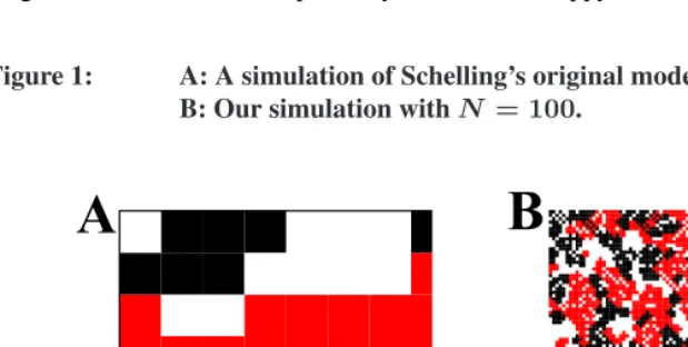
space for these models is the N×N square lattice with periodic boundary conditions (opposite sides identified). We consider two distinct populations, that, in Schelling’s words, refer to “membership in one of two homogeneous groups: men or women, blacks and whites, French-speaking and English speaking, officers and enlisted men, students and faculty, surfers and swimmers, the well dressed and the poorly dressed, and any other dichotomy that is exhaustive and recognizable” (Schelling 2006). We denote by B (black squares) and R (red squares, appear grey on black and white printing) these two populations. See Fig. 1. Together these agents fill up some of the N2 sites, with
V remaining vacant sites (white squares). Each agent has eight nearest neighbors, cor-responding to Moore, or Queen, neighborhood. Different neighborhoods were studied in different papers (see, e.g, Fossett 2006; Clark and Fossett 2008, where the size of the neighborhood was referred to as ‘vision’). Fix adisparate neighbor comfort threshold
T ∈ {0,1, . . . ,8}, and declare that a B or R ishappyifT or more of its nearest eight neighbors are B’s or R’s, respectively. Else, it is unhappy.
Figure 1: A: A simulation of Schelling’s original model withN = 8; B: Our simulation withN = 100.
Demographically, the parameterN controls the size of the city,v =V /N2controls
the population density or theoccupancy ratio(BusinessLocate 2009), andTis an “agent comfort index” that quantifies an agent’s tolerance to living amongst disparate nearest neighbors.
In choosing the algorithm of evolution we followed the protocol introduced in the original Schelling paper (Schelling 1969) and later used in Portugali, Benenson, and Omer (1994) and Benenson et al. (2006). We begin the evolution by choosing an initial con-figuration (described in Sect. 3) and randomly selecting an unhappy B and a vacant site surrounded by at leastT nearest B neighbors. Provided this is possible, interchange the unhappy B with the vacant site, so that this B becomes happy. We then randomly select an unhappy R and a vacant site having at leastT nearest neighbors of type R. Provided this is possible, we interchange the unhappy R with the vacant site, so that R becomes happy. We repeat this iterative procedure, alternating between selecting an unhappy B and an unhappy R, until afinal stateis reached, where no interchange is possible that increases happiness. For some final states, some (and in some cases, many) agents may be unhappy, but there are no allowable switches.
For the sake of completeness, we carried out simulations using other agent selection protocols, including random selection schemes. We observed no significant differences in the final states using the other selection schemes. This supports the claim in Young (1998) that the fine details of the evolution have negligible influence on the structure of the final states.
2. Schelling’s segregation is a small city phenomenon
Schelling considered the cases city sizeN = 8, neighbor comfort thresholdT = 3, and vacancy ratiov = 33%. ForT = 3or4, andv = 0, a “checkerboard" configuration of B’s and R’s (imagine placing B’s on the red squares and R’s on the black squares of an actual checkerboard) is a final state, since all agents have four like nearest neighbors.
The final state of a typical run of Schelling’s original model system is presented in Fig. 1A. Schelling performed many simulations by hand using an actual checkerboard, and observed that the final states presented a significant degree of global aggregation. He equated the global aggregation with segregation of a city.
In this paper, we investigate whether the global aggregation that Schelling observed for very small lattices persists for larger lattices. In Fig. 1B, we present a characteristic final state for our simulations with city sizeN = 100. Comparing Figs. 1Aand 1B, one can see a striking qualitative difference between the two final states. While there is some local aggregation in the final state withN = 100, there is no global aggregation. Visually inspecting this and other final states, one immediately sees that the global aggregation observed by Schelling is a small lattice phenomenon.
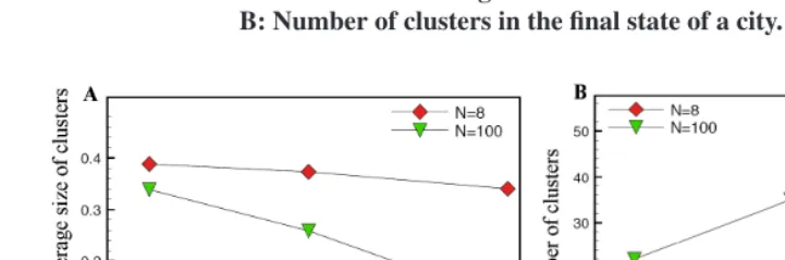
To quantify the difference in aggregation between a small city (N = 8) and a larger city (N = 100) we used a combination of two aggregation measures: the number of clus-ters in the final state of the model and the normalized average size of individual clusclus-ters (see Sect. 4.1 for a detailed description of these and several other measures of aggrega-tion). We determine the normalized average size of a cluster by dividing the average size of a cluster by the total number of agents in the city. The latter determines the proportion of a city covered by an individual cluster and provides a way to compare aggregation be-tween cities of different sizes. Figure 2 shows the mean values of these two aggregation measures in the final states of cities of two sizes (N = 8and100). We compute the mean values of the two measures based on100trials for each choice of the vacancy ratiovand neighbor comfort threshold T = 3. We observe that the normalized average size of a cluster in the large city is smaller than one in a small city. This implies that an individual cluster in a large city covers a smaller proportion of the city as compared to a cluster in a smaller city. Most final states of the small city are segregated into two clusters for all choices of the vacancy ratio while the number of clusters in the large city increases from
22for a city with24% empty locations to55for a city with33%empty locations. As we move from a small city to a large one, the relative size of a cluster in the final state decreases and the number of clusters increases. This shows that the large scale global aggregation observed by Schelling is strictly a small city phenomenon and does not occur for larger cities.
Figure 2: Aggregation measures to distinguish between a small city (N = 8) and a large city (N = 100) for constant neighbor comfort thresh-oldT = 3and different values of vacancy ratiov.
A: Normalized average size of an individual cluster. B: Number of clusters in the final state of a city.
3. Simulations
the number of R agents surrounding each agent in the city simultaneously. In our ‘city matrix’, an R agent is represented by 1, a B agent by -1 and an empty location by 0. Therefore, the problem of determining the number of surrounding R agents is reduced to adding up the 1’s in the neighborhood of each agent and ignoring the -1’s. We ignore the -1’s by simply finding the absolute value of each element in the city matrix; this converts the -1’s into 1’s but leaves the 1’s and 0’s unchanged. We call this modified matrix the ‘absolute value matrix’. When we add the city matrix and the absolute value matrix, all the -1’s are gone and the sum of all the elements gives the number of R agents in the 8-point neighborhood. Similar methods can be used to speed up the process of finding suitable locations for unhappy agents and computing aggregation measures.
We study the dynamics for large lattices and present our results mostly for city sizeN = 100. Figures 2-7 are all based on N = 100. In the last section, we discuss the cases
N = 50andN = 200, and show thatNgreater than100does not lead to qualitatively or quantitatively different states and phenomena. We restrict our discussion to cities having an equal number of B’s and R’s. We will report the results on the dynamics with different proportions of B’s and R’s in a separate manuscript (Singh, Vainchtein, and Weiss 2009). We consider neighbor comfort thresholdT = 3,4,5and vacancy ratiovbetween2%
and33%. The system does not evolve very much for other values ofT: forT = 1,2
almost all of the agents are satisfied in most of the initial configurations, while forT ≥6
there are almost no legal switches. Values ofvlarger than33%correspond to unrealistic environments. For each pair of parametersT andv, we perform100simulations. This number of simulations was chosen to ensure a95% confidence interval for parameter estimation. The Central Limit Theorem provides confidence intervals for the mean values of the aggregation measures.
We choose the initial configuration by starting with a checkerboard with periodic boundary conditions. Demographically, a checkerboard configuration is a maximally in-tegrated configuration. We then randomly remove half the intended vacant locationsv/2
of both B’s and R’s (thus keeping equal numbers of both agents). We randomly permute agents in two3×3blocks. Alternatively, we could choose a completely random initial configuration. In general, except for small values ofv, the final states are quantitatively similar to the ones obtained using the Schelling-like initial conditions.
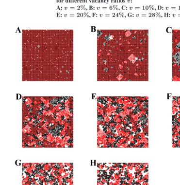
Figure 3: Characteristic final states for neighbor comfort thresholdT = 3 for different vacancy ratiosv:
A:v= 2%, B:v= 6%, C:v = 10%, D:v = 15%, E:v = 20%, F:v = 24%, G:v = 28%, H:v = 33%.
A
B
C
D
E
F
Figure 4: Characteristic final states for neighbor comfort thresholdT = 4 for different vacancy ratiosv:
A:v = 2%, B:v = 6%, C:v = 10%, D:v = 15%, E:v = 20%, F:v = 24%, G:v = 28%, H:v = 33%.
A
B
C
D
E
F
Figure 5: Characteristic final states for neighbor comfort thresholdT = 5 for different vacancy ratiosv:
A:v= 2%, B:v= 6%, C:v = 10%, D:v = 15%, E:v = 20%, F:v = 24%, G:v = 28%, H:v = 33%.
A
B
C
D
E
F
4. Analysis
4.1 Measures of Aggregation
In Figs. 3-5, aggregation appears to be a multifaceted phenomenon. One can observe that the states are visually quite different. However, to draw any quantitative conclusions and to arrive to any meaningful demographic observations, we need several measures (or in-dices) to describe the states. We begin the current section by defining several measures of aggregation that enable us to quantify this observation. In his papers, Schelling used two measures of aggregation:
1. The ratio of unlike to like neighbors that is called the[u/l]-measure. For a site on the lattice with coordinates(i, j)we define:
[u/l]i,j =qi,j+wi,j
si,j ,
wheresi,j,qi,j, andwi,jare the number of like, unlike, and vacant neighbors of the
agent located at(i, j), respectively. We define thesparsityh[u/l]iof a cluster by averaging the[u/l]-measure over the given cluster.
2. The number of agents that have neighbors onlyof the same kind (note that this definition excludes the vacant spaces as well). The abundance of such agents in-dicate the presence of large, “solid” clusters. This quantity is the most useful in quantifying between the states withT = 3andT = 4. We call the latter quantity seclusivenessand denote byN0.
Since the publication of Schelling’s papers, sociologists have devised new measures to quantify different aspects of segregation, including: evenness, exposure, cluster-ing, concentration and centrality (Duncan and Duncan 1955; Massey and Denton 1988; Massey, White, and Phua 1996). Exposure relates to the degree of contact between agents of different kinds and clustering relates to the degree of contiguity among agents of one kind. In this paper we concentrate on the exposure and clus-tering aspects of segregation. Along with Schelling’s two measures of exposure, we introduce an additional measure of exposure, as well as two measures of clustering.
A key observation is thatpis aLyapunov function, i.e., a function defined on every configuration which is strictly decreasing along the evolution of the system until it reaches a final state. Thus the system evolves to minimize the adjusted interface between the R and B agents. The final states are precisely the local minimizers of the Lyapunov function, subject to the threshold constraint. This Lyapunov function is also the Hamiltonian for a related spin lattice system related to the Ising model (Simon 1993). Such a notion ofpwas motivated by analogies of these models with the physics of foams. Note that for wedge-like utility functions, such as the ones considered in (Zhang 2004),pis not a Lyapunov function, even in the absence of noise.
Let us show that in the process of evolution every legal switch makesP smaller. Suppose we switch an R and a V. Before the switch, suppose R hadB1,R1, and
V1, of B, R, and V neighbors, respectively. Similarly, the numbers for the V agent
areD2,R2, andV2. Then the value ofP before and after the switch are:
Pinitial= 2B1+V1+B2+R2; Pf inal= 2B2+V2+B1+R1.
Thus,
Pf inal−Pinitial=B2+V2+R1−(B1+V1+R2).
Taking into account thatB1+V1+R1=B2+V2+R2= 8, we arrive at
Pf inal−Pinitial= 2 (R1−R2)<0.
Similarly, if the switch between R and B, we have
Pf inal−Pinitial= 2 (R2−R1) + 2 (B1−B2)<0.
The main consequence of the presence of a Lyapunov function is that it guarantees the convergence of the Schelling model to a final steady state. Moreover, sinceP
decreases by at least2on every switch andP cannot be negative, there can only be finitely many moves before the algorithm converges to an equilibrium state.
5. The total number of clusters in a configurationNC.This intuitively appealing
mea-sure of aggregation is useful to describe final states having mostly large compact clusters. For such systems,NCandLare the quantities that attract the viewer’s
at-tention first. To see its limitation, observe that “the maximally integrated” checker-board configuration withv = 0has just1 + 1 = 2clusters. The reason for that is that if two squares are considered to belong to the same cluster if they touch by a side or a vertex, clusters may be intermingled. The quantityNCis the most useful
for configurations consisting of compact clusters of a similar size. To study config-urations such as the final states forT = 5, a more useful quantity is the number of clusters that have greater then, say,Mmax/10agents, whereMmaxis the number
of agents in the largest cluster of a given kind.
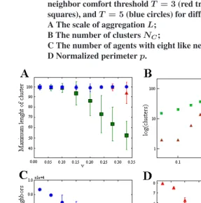
In Fig. 6, we plot average values of aggregation measures (2)-(5) introduced above for the final states withT = 3,4,5and several values ofv. The linear relationships of these disparate aggregation measures on population density seem remarkable. Often there is some deeper meaning behind such linear scaling, such as critical exponents in phase transitions, that may lead to construction of theoretical explanation of the phenomena.
4.2 Global aggregation dependence on the neighbor comfort thresholdT
From Figs. 3-5, one observes that:
1. the final states with neighbor comfort thresholdT = 3are very sparse, with a great deal of interweaving between both kinds of agents and vacant spots;
2. the final states withT = 4consist of compact clusters (that look like solid objects); and, finally,
3. the final states withT = 5consist of one (for each type) huge cluster together with a small number of remaining agents scattered around.
Varying the densityvdoes not radically alter the qualitative structure of the final states. We now quantify the aggregation for each value ofT, asvvaries between2%and33%.
4.2.1 T=3: sparse clusters
Figure 6: Statistics of four key measures of aggregation of final states for neighbor comfort thresholdT = 3(red triangles),T = 4(green squares), andT = 5(blue circles) for different vacancy ratiov: A The scale of aggregationL;
B The number of clustersNC;
C The number of agents with eight like nearest neighborsN0;
D Normalized perimeterp.
The sparsity of the final states withT = 3is due, in part, to large blocks of the initial checkerboard configuration that remain unchanged during the evolution. We call this phenomenon thesuper-stabilityof the checkerboard. Every agent is not just happy, but has one like neighbor to “spare”. Thus, it takes a large perturbation to make a given agent move and, therefore, only agents close to the initially perturbed sites move. Consequently, Schelling required a large density of vacant spacesv (33%) to overcome checkerboard super-stability. Following the panels of Fig. 3, one can see that asvdecreases, larger and larger parts of the initial configuration remain unchanged during the evolution.
result in larger clusters, and thus lead to greater global aggregation. The number of clus-ters in the final states, NC, decreases as v decreases (Fig. 6B) and the dependence is
almost cubic. The value for the slope in Fig. 6Bcorresponding toT = 3is2.86and the value3is well within the error bars. We can group the cubic dependence of the number of clusters and the previously noted linear dependence of aggregation measures on pop-ulation density under the category of scaling laws. We use the term “scaling law” in the same sense as it is used in physics and biology: as a particularly simple relation (e.g., linear, cubic, etc.) between two important variables. Often there is deep science behind scaling laws (such as critical exponents in phase transitions and species-area relationships in ecology) and attempts to explain them often lead to a theoretical explanation of the phenomena.
The seclusiveness measure, N0, is a monotonically decreasing function ofv: asv
decreases, the final state approaches the checkerboard and, naturally, almost all the agents have some contacts with other agents. Similarly, the smaller the value ofv, the larger the normalized perimeter,p. The values ofparound4for large values ofvindicate that most of the agents have in their 8-point neighborhoods around2−3vacancies and1or2agents of a different kind. This conclusion is supported by the visual inspection of Fig. 3F-H. Therefore, the low comfort threshold results for an individual agent in the presence of the vacancies in the neighborhood, rather than the agents of a different kind.
4.2.2 T=4: compact clusters and mesoscale aggregation
In Fig. 4 we present typical final states for neighbor comfort thresholdT = 4and different values of vacancy ratiov. IncreasingT from3 to4eliminates the checkerboard super-stability phenomenon and results in strikingly different structures of aggregation in final states. Namely, every final state consists of relatively small number of compact clusters, that clearly depends onv.
For relatively large values ofv, such final states exhibitmesoscale aggregationand, for small values ofv,macroscale aggregation. There seems to be no canonical way to separate the two types of aggregation. Our criterion is to define the transition when the size of the largest cluster,L, becomes equal toN.
report living in a “dense” conditions (no vacancies in the neighborhood), while the vacant spots create patches of their own.
One can see in Fig. 6Dthat the characteristic values ofpare at most2for all the values ofv. It indicates that most of the agents have in their 8-point neighborhoods just1−2
vacancies and no agents of a different kind. This conclusion is supported by the visual inspection of Fig. 4F-H. Thus, for the low comfort thresholdT = 4there are almost no contacts between the agents of a different kind.
In addition to the seclusiveness,N0, we quantify the differences in the final states for
neighbor comfort thresholdT = 4with vacancy ratio v ranging fromv = 33%down tov = 2%, with three measures: the number of clusters,NC, the scale of aggregation,
L, (Fig. 6). By providing opportunities for increasingly “easier satisfaction," one might believe that decreasingvincreases the values of number of clustersNC. In other words,
when there are a lot of vacancies, agents have many choices and it leads to appearance of many small “islands". Our study confirms this, and the dependence is remarkably linear. The value for the slope in Fig. 6Bcorresponding toT = 4is0.89and the value1is well within the error bars. Specifically, for typical final states withT = 4,v= 33%(Fig. 4H)
NC is relatively high; forT = 4, v = 15%, NC is smaller (Fig. 4D) and the clusters
on average are bigger; finally, states withT = 4,v = 2%contain only a few compact clusters of either type that stretch across the whole lattice (L = 100). In general, asv
decreases,Lincreases almost linearly (see Fig. 6A).
Thus forT = 3 andT = 4, the increase inv leads to the opposite effects: they increaseanddecreasethe level of global aggregation, respectively.
4.2.3 T=5: final states with many unhappy agents
For small vacancy ratiov, the dynamics with neighbor comfort thresholdT = 5always results in a final state achieved after just a few switches, and consists of mostly unhappy agents with no vacant space to where they could move. However, a slight modification of the selection algorithm to allow direct R-B switches (similar to the selection algorithms in (Pollicott and Weiss 2001; Weisbuch et al. 2002; Zhang 2004)), results in significant global aggregation and drastically reduces the number of unhappy agents, although not eliminating them entirely. The presence of unhappy agents in the final states is a new phe-nomenon, which we do not observe in simulations forT = 3(while such configurations theoretically exist, they are extremely unlikely) and is much less pronounced forT = 4.
In Fig. 5 we present typical final states for neighbor comfort thresholdT = 5 and different values of vacancy ratiov with modified selection algorithm. A typicalT = 5
increases (see Fig. 7B). Another clear indication of the growth of the main cluster is the increase of the number of agents with 8 similar neighbors,N0, illustrated in Fig. 6C.
The globally aggregated final states (small values ofv) withT = 5(with modified selection) andT = 4(with Schelling selection) appear similar in terms of the number of large clusters and the scale of aggregation,L(Figs. 5Aand 4A). However, there is a large difference in their adjusted perimeterp: it is much smaller for neighbor comfort threshold
T = 5 (see Fig. 6D). There are two reasons for smallerp. First, the clusters are more “circular”, thus reducing the perimeter-to-area ratio. Second, there are almost no vacant spots inside the clusters forT = 5: almost all the vacant spots are located at the boundary between theRandBclusters.
Figure 7: Statistics of the final states with neighbor comfort thresholdT = 5:
A: The average number of unhappy agents in final states; B: The average number of the agents in the two big clusters.
The average number of unhappy agents in final states for different values ofT and
thresholdT and vacancy ratiov. ForT = 3,v = 33%; T = 4,v = 33%; T = 4,
v = 2%; andT = 5,v = 2%the average number of steps are3596,5192,5573,4422, respectively. The switches forT = 5,v = 2%that included both R and B agents are counted twice. The most striking feature is that it takes significantly fewer switches to achieve the final state forT = 5than forT = 4. In Fig. 8 we present the distribution of the number of jumps for different agents.
5. Final states with
N
=
50
,
N
=
100
and
N
=
200
To illustrate the dependence of the final states of city sizeN, we performed100 simula-tions forN = 50,N = 100andN = 200. In Figs. 9-11 we present characteristic final states forN = 50,N = 100, andN= 200, respectively. One can see that the figures for
N= 50andN = 200are qualitatively very similar to Fig. 10.
In Fig. 12 we present characteristic plots of two of the aggregation measures (namely the perimeter and the number of agents with only like neighbors) for city sizeN = 50,
N = 100, andN = 200. One can see that all three columns are very similar to each other.
Figure 9: Characteristic final states forN = 50and different values of neighbor comfort thresholdTand vacancy ratiov:
A:T = 3,v = 2%, B:T = 3,v = 15%, C:T = 3,v = 33%, D:T = 4,v = 2%, E:T = 4,v = 15%, F:T = 4,v = 33%, G:T = 5,v = 2%, H:T = 5,v = 15%, I:T = 5,v= 33%.
A
B
C
D
E
F
Figure 10: Characteristic final states forN = 100and different values of neighbor comfort thresholdT and vacancy ratiov:
A:T = 3,v = 2%, B:T = 3,v = 15%, C:T = 3,v= 33%, D:T = 4,v = 2%, E:T = 4,v = 15%, F:T = 4,v = 33%, G:T = 5,v = 2%, H:T = 5,v = 15%, I:T = 5,v = 33%.
A
B
C
D
E
F
Figure 11: Characteristic final states forN = 200and different values of neighbor comfort thresholdTand vacancy ratiov:
A:T = 3,v = 2%, B:T = 3,v = 15%, C:T = 3,v = 33%, D:T = 4,v = 2%, E:T = 4,v = 15%, F:T = 4,v = 33%, G:T = 5,v = 2%, H:T = 5,v = 15%, I:T = 5,v= 33%.
A
B
C
D
E
F
Figure 12: Characteristic values of the perimeter (top row) and the number of agents with only like neighbors (bottom row) forN = 50(left column),N = 100(middle column), andN = 200(right col-umn) different values of neighbor comfort thresholdTand va-cancy ratiov; in every frame,T = 3(red triangles),T = 4(green squares), andT = 5(blue circles).
6. Concluding remarks and acknowledgements
combination of the disparate neighbor comfort threshold and the number of vacancies in a city, in particular that aggregation is an increasing function of vacancies whenT = 3
but is inversely correlated with vacancies whenT = 4. We also find a remarkable linear dependence of aggregation measures on the vacancy ratio in large cities.
References
Benenson, I., Or, E., Hatna, E., and Omer, I. (2006). Residential Distribution in the City – Reexamined. 9th AGILE International Conference on Geographic Information Science (April 2006).
Bruch, E. and Mare, R. (2006). Neighborhood Choice and Neighborhood Change. Amer-ican Journal of Sociology112(3): 667–709.doi: 10.1086/507856.
BusinessLocate (2009). Occupancy ratio. Http://www.realestateagent.com/glossary/real-estate-glossary-show-term-1699-occupancy-ratio.html.
Clark, W. (1986). Residential segregation in American cities: A review and interpretation. Population Research and Policy Review5(2): 95–127. doi: 10.1007/BF00137176. Clark, W. (1991). Residential Preferences and Neighborhood Racial Segregation: A Test
of the Schelling Segregation Model.Demography28(1): 1–19.doi: 10.2307/2061333. Clark, W. (1992). Residential preferences and residential choices in a multiethnic context.
Demography29(3): 451–466.doi: 10.2307/2061828.
Clark, W. and Fossett, M. (2008). Understanding the social context of the Schelling segregation model.Proceedings of the National Academy of Sciences105(11): 4109– 4114.doi: 10.1073/pnas.0708155105.
Duncan, O. and Duncan, B. (1955). A Methodological Analysis of Segregation Indexes. American Sociological Review20(2): 210–217. doi: 10.2307/2088328.
Fossett, M. (2006). Ethnic Preferences, Social Distance Dynamics, and Residential Seg-regation: Theoretical Explorations Using Simulation Analysis. The Journal of Mathe-matical Sociology30(3): 185–273.doi: 10.1080/00222500500544052.
Gerhold, G., Glebsky, G., Schneider, C., Weiss, H., and Zimmermann, B. (2008). Computing the complexity for Schelling segregation models. Communications in Nonlinear Science and Numerical Simulation 13(10): 2236–2245. doi: 10.1016/j.cnsns.2007.04.023.
Laurie, A. and Jaggi, N. (2003). Role of ’Vision’ in Neighbourhood Racial Segregation: A Variant of the Schelling Segregation Model.Urban Studies40(13): 2687–2704.doi: 10.1080/0042098032000146849.
Massey, D. (1990). American Apartheid: Segregation and the Making of the Underclass. American Journal of Sociology96(2): 329–357. doi: 10.1086/229532.
Massey, D., White, M., and Phua, V. (1996). The Dimensions of Segrega-tion Revisited. Sociological Methods & Research 25(2): 172–206. doi: 10.1177/0049124196025002002.
Oliphant, T. (2006).A Guide to NumPy. Trelgol Publishing.
Pollicott, M. and Weiss, H. (2001). The Dynamics of Schelling-Type Segregation Models and a Nonlinear Graph Laplacian Variational Problem. Advances in Applied Mathe-matics27(1): 17–40.doi: 10.1006/aama.2001.0722.
Portugali, J., Benenson, I., and Omer, I. (1994). Sociospatial residential dynamics: stabil-ity and instabilstabil-ity within a self-organizing cstabil-ity.Geographical Analysis26(4): 321–340. Sander, R., Schreiber, D., and Doherty, J. (2000). Empirically Testing a Computational Model: The Example of Housing Segregation. Proceedings of the Workshop on Simu-lation of Social Agents: Architectures and Institutionspp. 108–115.
Schelling, T. (1969). Models of segregation.American Economic Review59(2): 488–493. Papers and Proceedings of the Eighty-first Annual Meeting of the American Economic Association (May, 1969).
Schelling, T. (1971a). Dynamic models of segregation. Journal of Mathematical Sociol-ogy1(1): 143–186.
Schelling, T. (1971b). On the ecology of micromotives. The Public Interest25: 61–98. Schelling, T. (2006).Micromotives and macrobehavior. New York: W.W. Norton. Simon, B. (1993).The statistical mechanics of lattice gases. Princeton University Press. Singh, A., Vainchtein, D., and Weiss, H. (2009). Schelling’s Segregation Model with
Minorities .
Vinkovic, D. and Kirman, A. (2006). A physical analogue of the Schelling model. Proceedings of the National Academy of Sciences 103(51): 19261–19265. doi: 10.1073/pnas.0609371103.
Weisbuch, G., Deffuant, G., Amblard, F., and Nadal, J. (2002). Meet, discuss, and segre-gate! Complexity7(3): 55–63.doi: 10.1002/cplx.10031.