in the population sciences published by the Max Planck Institute for Demographic Research Konrad-Zuse Str. 1, D-18057 Rostock · GERMANY www.demographic-research.org
DEMOGRAPHIC RESEARCH
VOLUME 10, ARTICLE 7, PAGES 171-196
PUBLISHED 11 MAY 2004
www.demographic-research.org/Volumes/Vol10/7/
DOI: 10.4054/DemRes.2004.10.7
A Research Article
published in honor of Eugene A. Hammel
Tracing Very Long-Term Kinship
Networks Using SOCSIM
Mike Murphy
1 Introduction 172
2 Data and methods 175
3 The populations used 176
4 Analytic, empirical and operational questions 178
5 Results of the analysis 180
5.1 Probability of no descendant 180 5.2 Number of distinct descendants 181 5.3 The concept of generations and long-term
replacement
184
5.4 Degree of relatedness 186
6 Summary and conclusions 188
7 Acknowledgements 189
Notes 190
References 191
A Research Article
published in honor of Eugene A. Hammel
Tracing Very Long-Term Kinship Networks Using SOCSIM
Mike Murphy1
Abstract
While each individual has 10 billion ancestors a thousand years ago, these are not distinct and the actual number of distinct ancestors is much smaller. A female (‘Mitochondrial Eve’) and a male ancestor (‘Y-chromosome Adam’) of all humans certainly existed, possibly about 100,000 years ago, and a most recent common ancestor (‘MRCA’) of all humans existed much more recently. I use the SOCSIM micro simulation program to examine the patterns of descent over periods of several centuries of an initial population using as indicators: the proportion of these people without any living descendants by the end year of the analysis; the mean value and variability in the number of their distinct descendants; and the distribution of genetic contribution (ie the expected proportion of the DNA of individuals in the initial population found in the later population). About three-quarters of those born in the past have no descendant, mainly because they did not reach the age of reproduction. With the initial population sizes used here, about 4,000 people, after about 500 years the number of descendants of all of those who have any descendant becomes close to the size of the total number of descendants, confirming that even in this time-scale, a person is either the ancestor of everyone, or of no-one. However, the genetic contribution that those in the initial population make to later generations does not exhibit a similar tendency to uniformity. Issues such as the sensitivity of simulation results, which are inevitably based on smaller numbers than real human breeding group sizes, and the need to modify conventional measures of generational replacement to cases with multiple lines of descent are also considered.
1
1.
Introduction
The first page of Preston, Heuvaline and Guillot (2001, p1) defines the scope of the discipline of demography: ‘Demographers also use the term “population” to refer to a … collectivity that persists through time even though its members are continuously changing through attrition and accession. This collectivity persists even though … a virtually complete turnover of its members occurs at least once a century. Demographic analysis focuses on this enduring collectivity’. However, in practice a very small fraction of demographic work is concerned with such long-term population movements, and much is concerned with relationships at a single point of time. While there have been valuable demographic studies of long-term aggregate population trends (eg Wrigley and Schofield 1981), studies of the dynamics of populations ‘continuously changing through attrition and accession of individuals’ are very rare, in part because of the lack of information to track patterns of descent over long periods of time. Therefore, empirical studies have tended to be undertaken by groups such as genealogists or geneticists usually for the specialised and atypical populations for which relevant information is available. The lack of demographic interest is surprising, since so much demographic analysis is concerned with the patterns of numbers of offspring of women (including childlessness), but so little with the numbers of offspring in the next generation of grandchildren, and almost none in patterns among generations further apart, as databases such as POPLINE confirm. However demography has developed a number of approaches for the analysis of the dynamics of human populations that may be combined with those of these neighbouring disciplines to elucidate the long-term dynamics of population in greater detail than hitherto. In this paper, I bring together such approaches within the framework of a demographic microsimulation model, SOCSIM, and present some findings about long-term individual-level patterns of descent. These results may be used to compare and to complement those from the other main disciplines that have been concerned with some aspects of long-term population dynamics, including mathematical statistics, where powerful, but highly artificial, models have been developed for well over a century, and I show how recent results from stochastic theory are related to those in demographic anthropology (Wachter and Laslett 1978).
usually requires modelling. A given person today has 2q ancestors q generations ago, so that with an average 30-year generation period, 1000 years ago, the number of ancestors is over 10 billion at a time when the global population was under one billion and lack of geographical mobility means that the actual pool of ancestors is much smaller than the global figure (Table 1). Although each of these 10 billion is a real person, in that a direct line of descent that can be drawn from the descendant to the ancestor, they are not distinct and the same ancestor will appear on many different occasions since there will usually be many links between two ancestors separated by long distances in time.
Table 1: Number of ancestors (non-distinct)
Generations Years Population size
0 0 1
1 30 2
5 150 32
10 300 1,024
15 450 32,768
20 600 1,048,576
25 750 33,554,432
30 900 1,073,741,824 35 1050 34,359,738,368
Note: this Table also gives the numbers of descendants if each individual has two children who survive to themselves reproduce.
patterns arises, including pedigree studies, which have been a principal method for identifying rare recessive diseases in particular (Dawkins 1992; Jones 1992, 1996). A recent DNA-based study suggested that a descendant of a 9,000 year old skeleton (‘Cheddar man’) found in England was living in same location (Sykes 2001).
In any population, the number of mothers of daughters is less than the number of females in the next generation (Note 1). Therefore the further back one goes, the numbers decrease until there is only one such female, often called ‘Mitochondrial Eve’, because mitochondrial DNA (which is in organelles outside the cell nucleus, and is essentially transmitted only through the mother’s egg) is therefore inherited through the maternal line (Ayala 1995; Cann, Stoneking and Wilson 1987; Vigilant et al 1991). Correspondingly, since the Y-chromosome is passed only through the father, a directly analogous argument shows the existence of ‘Y-chromosome Adam’. The dates of these ancestors are typically set at around 100,000 years age (Pääbo 1995; Dorit, Akashi and Gilbert 1995), with Y-chromosome Adam being assumed to be rather more recent than Mitochondrial Eve since there is greater variability in male than in female reproductive performance. There is, of course, no suggestion that these formed a couple, and they almost certainly did not.
Recently analytic studies have investigated the issue of common ancestry from a two-sex perspective (Chang, 1999), that goes beyond the earlier single sex of descent models. A more sophisticated concept is that of ‘Most recent common ancestor’ (MRCA) (Chang, 1999), which refers to descent through any line, and figures of the order of 1,000 to 3,000 years ago for this common ancestor have been suggested, although this is probably an underestimate because it is based on the assumption of a randomly mating, non-overlapping generations, homogeneous population, which does not distinguish two sexes. He shows that the number of generations back to this MRCA for a population of size n is only log2(n), giving a value of 32.5 generations (or 975
years ago) for a global population of size 6 billion. Chang (1999, p 1005) notes that ‘an application to the world population of humans would be an obvious misuse’ of the model.
billion distinct ancestors a millennium ago, only one of those born around that time would be in a direct female line.
The range of numbers of ancestors at earlier times quoted above represent the maximum and minimum indicators of long-term patterns of descent. These studies are often based on theoretical and simplified models and they do not, for example, take account of actual patterns of human reproduction, including population heterogeneity, and they do not show the evolution of such kinship linkages in real human populations. Therefore, in this paper, I have undertaken some preliminary work in constructing counts of the number of ancestors and descendants of a population over long periods of time (at least in comparison with most demographic studies) with a demographic regime broadly that of Britain using the SOCSIM micro simulation program in order to assess the possibilities of such approaches, which as Chang (1999) notes, will be necessary to provide realistic models to complement theoretical ones.
2. Data and methods
Demographic micro simulation is the principal method used to elucidate kinship patterns in historical, contemporary and future populations (Smith 1987; Wachter 1987; Wolf 1994; Zhao 1996; Van Imhoff and Post 1998). This analysis uses the SOCSIM demographic micro simulation model, originally developed by Gene Hammel and Ken Wachter at Berkeley with Peter Laslett at Cambridge University (Hammel, Wachter and Laslett 1978; Hammel, Mason and Wachter 1990), in which an initial population is subject to appropriate rates of fertility, mortality and nuptiality (including divorce). In recent decades, cohabitation has become increasingly important and it is also included in the model (Murphy, 2001).
computationally efficient and freely available so that the code can be amended or extended by users, in this case to generate the specific types of links between individuals.
3. The populations used
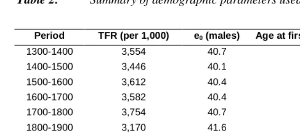
The model starts with an initial population that evolves under the given rates of fertility, mortality and nuptiality. The initial populations are of sizes of 4,000 and 10,000, with the age structure of England in 1741 taken from Wrigley and Schofield (1981). Two simulation periods of 600 years were chosen: 1250 to 1850, and 1750 to 2350. The first demographic regime was that of a pre-industrial (and pre-transitional) society using demographic rates provided by the Cambridge Group for the History of Population and Social Structure. These pre-transitional rates, which refer to the period around 1700 to 1750, are assumed to hold over the whole period 1250 to 1850, since the values for earlier periods were not very different and they provide a realistic set of rates with a long-term growth rate close to zero. These baseline values, shown in Table 2, lead to a population with a small but positive rate of growth (‘unconstrained’ values) and I also use a second set with fertility values slightly adjusted to make the long-term population growth rate close to zero (‘constrained’ values).
Table 2: Summary of demographic parameters used
Period TFR (per 1,000) e0 (males) Age at first marriage (males)
1300-1400 3,554 40.7 29.5
1400-1500 3,446 40.1 29.6
1500-1600 3,612 40.4 28.8
1600-1700 3,582 40.4 29.5
1700-1800 3,754 40.7 29.2
1800-1900 3,170 41.6 29.1
1900-2000 2,096 63.6 28.1
2000-2100 2,122 76.4 32.4
2100-2200 2,139 76.5 32.5
2200-2300 1,996 76.4 33.0
Note: constrained values for period 1300-1800.
Beyond 2000, the TFR is assumed to be rather higher than at present in Britain and most industrialised countries, but current rates would lead to a population too small for useful analysis by 2350. Mortality is expected to continue to improve and the average age at marriage to increase.
The partnership algorithm is based on a ‘marriage market’ that those adults who are not currently married join in order to seek a partner from the pool of eligibles of the opposite sex. People enter the pool of eligibles according to the appropriate population age, sex and marital-status specific marriage rates. Partners are found by a scoring algorithm that has a preferred spousal age difference of about two years and with preferences being tapered, so that all partnerships are confined to cases in which the man is no less than five years younger or no more than ten years older than his partner. The model includes a prohibition on incest between siblings and parents and children. It is possible to specify alternative algorithms (eg Murphy 2003), which could include systems that promote marriage among kin, such as in traditional Japanese and some South Asian societies, or discourage it, such as the prohibition of marriage of those related up to the seventh degree by the Catholic Church in the eleventh century.
4. Analytic, empirical and operational questions
The first question is the feasibility of undertaking meaningful long-term simulations, given the very large number of relationships that build up as shown in Table 1. It was found necessary to develop an alternative kinship network structure to enable the multiple lines of descent to be analysed satisfactorily (discussed in the Appendix), and population sizes of up to 10,000 people and time periods of about 600 years are possible, although a single simulation can take some hours to run. While this limits the number of issues that can be addressed simultaneously, nevertheless some of alternative simulations were undertaken to assess the sensitivity of the results to different conditions. Different initial population sizes were chosen to assess the sensitivity of different breeding populations (demes, or isolate size). Real populations are not closed, although establishing the effective breeding size of human populations is problematic, and no obvious estimates were found for this analysis. However, Cavalli-Sforza and Bodmer (1971, p 482) quote a figure of 278 for the upper Parma Valley, in a relatively isolated area for this important, but admittedly somewhat arbitrary parameter. Urban populations have larger effective breeding group sizes, and therefore initial population sizes of 4,000 and 10,000 were chosen for these experiments. The distribution of descendants might also be expected to be sensitive to the rate of population growth, so alternative models were constructed with a slow rate of growth of 0.2% per annum (doubling time of about 350 years), and one in which the fertility rates were constrained to make the rate of growth close to zero.
For the 1250 start date, 5 models were run with initial population size of N: N=4,000 for 600 years (constrained)
N=4,000 for 600 years (unconstrained) N=4,000 for 300 years (unconstrained) N=10,000 for 300 years (unconstrained) N=10,000 for 300 years (constrained)
These alternatives were chosen to assess the sensitivity of the outcomes to the initial population size, the time interval, and to the demographic rates used. (For the 10,000 initial size population, I use a 300-year horizon because of machine constraints.)
initial population are those born in years 1300-15 (the ‘original population’) and the main group of descendants analysed are those born 500 years later, in years 1800-15. For the 1750 initial population, the corresponding original and descendant populations are those born in 1800-15 and 2300-15 respectively. A 15-year window provides sufficient numbers to make generalisations, but does not contain any parent-child combinations, since the minimum age at childbearing is over 15 years.
For each person in the original population, I determine the number of descendants - if any - in the target population. The degree of relatedness between an ancestor and a descendant is the sum of (0.5)q for all distinguishable lines of descent that connect them, where q is the number of generations separating them in a given lineage. The degree of relatedness gives the genetic contribution of the ancestor to his or her descendants’ genomes. The degree of relatedness plays a central role in the analysis of mechanisms of kin selection (Hamilton 1964a,b), and it may also be analogous to any form of inheritance that is divided between children independently of the number of children. If the population contains no inbreeding, then there is only one line of descent, but as noted above, this is clearly not the case and a main interest is in the distribution of degree of relatedness after many generations.
There are a number of indices of overlap of relationships in genetic studies, such as inbreeding coefficients, kinship coefficients, consanguinity and co-relatedness. The first is used widely but refers to an individual, the probability that he or she has inherited the same gene at a particular locus from a single ancestor (‘identical by descent’, or ibd), whereas I am concerned with more general patterns of flows between generations, and so I use degree of relatedness as the main indicator. Consideration of alternative indicators and of patterns of degrees of relatedness among living people will be deferred.
5. Results of the analysis
5.1. Probability of no descendant
About three-quarters of those born in 1300-15 have no descendant born in the period 1800-15 (Table 3, models 1 and 2). This figure is only slightly smaller for the growing than for the stationary population over the period, showing that the probability of having no descendant is relatively insensitive to population growth. More noteworthy is the fact that the proportion of those with no descendant at 500 years is identical to the figure found for that population after 250 years (models 1 and 3; note that in this case, the values are based on the same population analysed at two points of time). Thus if there is any descendant born about 250 years later, it is very likely that there will be descendants born a further 250 years ahead. The reason for this is that a given individual is likely to have a large number of descendants after a period of 250 years: an average of just over two children surviving to adulthood is necessary to keep population numbers constant and Table 1 shows that the average number of such descendants will be about 250 (not necessarily all distinct, but it is likely that there will be a large number of distinct descendants – the Table shows the numbers of children if two survive to reproduce themselves). Thus there are a large number of chances of having at least one descendant 500 years later if there are descendants after 250 years, since not do so would mean that every one of these descendants after 250 years would have to have no descendants, which become increasingly unlikely as the number of descendants increases. The chance of someone having no descendant after 500 years who had had 250 descendants 250 years later, each of whom had independent probabilities of about 0.75 of no descendant 250 years later is 10-31. Thus complete extinction essentially takes place in the first few generations, with the failure to reach the age of reproduction being the main determinant.
Table 3: Probability of no descendant born in future periods
Model Population born Years ahead
Initial population size & type
Probability Size of original population Number with descendants in original population Size of descendant population
1 1300-15 500 N=4,000 unconstrained 71.7 1,911 540 4,781
2 1300-15 500 N=4,000 constrained 75.9 1,837 443 1,814
3 1300-15 250 N=4,000 unconstrained 71.7 1,911 540 2,909
4 1300-15 250 N=10,000 unconstrained 72.8 5,035 1,369 8,195
5 1300-15 250 N=10,000 constrained 76.4 4,501 1,061 4,613
The difference in the probability of having no descendant after 250 years with the same demographic regime, but with different initial population sizes is very small and probably due to stochastic variability (models 3 and 4, or 2 and 5), suggesting that the results are insensitive to initial population size, which is not surprising since this is determined mainly by events in the early years of the simulation run, but emphasising that results can be generalised to larger populations and do not depend on a particular choice of initial population size. The probability of having a descendant in the more recent 500-year period is broadly similar (model 6), but this is because the initial demographic regime of the nineteenth century was superior to the pre-transitional one, rather than to the very different patterns of later periods.
5.2. Number of distinct descendants
The mean number of distinct descendants of those born in the period 1300-15 with at least one ancestor 250 years later with the constrained model was 270 (the value averaged over for all those in the original population was about one quarter of this) with this closed breeding group of total size 4,000, rather similar to the number if there was no inbreeding with the simple assumption of Table 1. However, more noteworthy is the fact that the number increases by only a factor of about seven over the next 250 years with a fixed population size, as the multiple lines of descent between individuals build up (Table 4). After 500 years, this average number is close to the total population size of the descendant population (and the descendant population size provides a ceiling). The average number of descendants is, of course, larger in a growing population (models 2 and 3), but rather similar in the two time periods (models 1 and 4). The key factors that determine the numbers of distinct descendants are (i) whether there is any descendant; (ii) the population growth rate; and (iii) the population breeding size.
Table 4: Mean number of descendants
Model Population born Years ahead Initial population size & type Mean of those with at least one descendant
1 1300-15 250 N=4,000 unconstrained 430
2 1300-15 500 N=4,000 unconstrained 4,709
3 1300-15 500 N=4,000 constrained 1,768
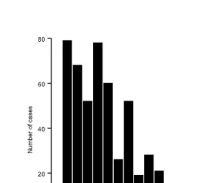
Figure 1(a): Estimated number of descendants: 1300-15 cohort after 250 years
These results are consistent with Chang’s (1999) theoretical model, which leads to the conclusion that before about 700 AD, every human is either an ancestor of everyone alive today, or has no live descendants. However, in contrast, to Chang’s model that about 80 per cent of people in the earlier period are the ancestors of everyone alive today, the figure here is about 25 per cent of births, largely because of mortality before reaching the age of reproduction (Note 2).
5.3. The concept of generations and long-term replacement
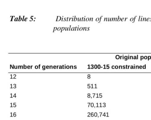
Almost all demographic analysis, descriptive and theoretical, is based on the concepts of time period and/or cohorts, and the relationship between these approaches remains a major interest of the discipline and such issues are relevant to neighbouring disciplines such as population genetics. As Shryock, Siegel and Stockwell (1976, p326) note: ‘In taking up generation reproduction rates, we are passing to measures of reproduction that are based on the fertility and mortality experience of an actual cohort of women during its reproductive years’, but key concepts such as intergenerational replacement, usually of mothers by their daughters, do not translate straightforwardly to the relationship spanning more than one generation. Even extensions to the relationship between fertility of grandparents and grandchildren are rare as noted in the first paragraph of this paper (Murphy and Wang 2001; Mueller 2001), although there are relatively few problems, since the assumption that each person has four distinct grandparents is reasonable, given the low estimates of incest (Cavalli-Sforza and Bodmer 1971). However, the concept of a well-defined number of generations between two given individuals is not meaningful for long-range analysis since the great majority of descendants will have a given ancestor through different numbers of generations, and the network formed is not a conventional genealogical one since a given individual can appear at different places in the genealogy, see the Appendix for a discussion. Table 5 shows that the mean number of links per person in these populations is between 1 and 2 thousand, and that the number of generations between an individual in the original and an individual in the descendant populations has a range of 12 to 20 for the 500-year periods. The average length of a generation is shorter in the earlier period, reflecting that later age at onset of childbearing assumed in the later period, but variability is less in the later period. However, in both cases, the two largest numbers of generations contain about three-quarters of all values.
generations between two people, and comparison between time periods would appear to be the most appropriate ways of analysing change, even though the limitations of period data are well-recognised. If a concept of generational length is to be retained, then it will be necessary to consider such variability in the same way that standard analysis has to do so. For example, variability in the age at childbearing leads to modifications in the equations of population dynamics as compared with the case of a fixed age. For example, the value of the intrinsic rate of growth r is approximated by the second order solution to Lotka’s equation (Keyfitz, 1968)
2r2σ2 - rµ + ln(R0)= 0
where R0 is the NRR, and µ is the mean and σ2 the variance of the childbearing distribution. If the age at childbearing was fixed (ie σ2 = 0), then r = ln(R0)/µ, but if it is not fixed (ie σ2 >0), then the annual population growth will be higher, although the
NRR and mean age are the same in both cases.
Table 5: Distribution of number of lines of descent between original and descent populations
Original population
Number of generations 1300-15 constrained 1800-15
12 8 0
13 511 0
14 8,715 112
15 70,113 4,087
16 260,741 44,187
17 334,155 165,709
18 103,228 264,920
19 5,571 85,052
20 32 3,755
Total 783,074 567,822
Average no. lines 1,768 1,088
Average length of generation
5.4. Degree of relatedness
An alternative way of analysing long-term kinship links is by the genetic contribution that the earlier generation makes to the later one. The degree of relatedness for a given line of descent between two people is (0.5)q, where q is the number of generations between the ancestor and descendant. Since many people will have a given ancestor through more than one line - in cases such as that of Table 5, many thousands - I sum these components (when cousins marry, no matter how widely separated, their offspring will have at least one ancestor in common, and the overall degree of relatedness is the fraction of genes identical by descent that the two individuals have in common).
Figure 2 shows the distribution of the sum of degrees of relatedness in the descendant population for each member of the original population who has a descendant for the period 250 and 500 years ahead (Figures 2(a) and 2(b)) (Note 3). In contrast to the results of Figure 1, this distribution does not show a tendency to collapse to a single value and, if anything, the variability tends to increase over time. The reason for this is that although the number of distinct descendants depends only on there being at least one line of direct descent, the degree of relatedness depends also on the number of links and the number of intervening generations. Thus even without any mechanism that favours one group, disparities remain effectively constant over time, when measured, for example, by the coefficient of variation.
Figure 2(b): Sum of degree of relatedness: 1300-15 cohort after 500 years
Figure 3: Distribution of degree of relatedness: 1300-15 cohort after 500 years
6. Summary and Conclusions
In this preliminary analysis, I have shown that the SOCSIM kinship microsimulation model can elucidate long-term demographic processes for which data are not available, and that some of the results although at first appearing counter-factual are consistent with other studies. These methods could be extended in a number of ways to include population mixing, additional patterns of heterogeneity and assortative mating to provide more realistic models. Since the full kinship network is available for analysis, it is possible to compute indices relating to the descendant population, such as degree of inbreeding, therefore providing a flexible and realistic model for investigating a range of issues related to patterns of inheritance. In order to do so, it was necessary to construct an alternative linked network to the conventional genealogical one, in order to make such analyses feasible with current technology.
reasonable, but in addition, it is shown that the results are usually relatively insensitive to the chosen population size.
While there has been considerable interest in macro-level demographic evolution (eg Wrigley and Schofield 1981), with exceptions such as Hajnal (1964, 1982) and Wachter (1978), demographers have had little interest in long-term micro-demographic processes, and they have often attempted to seek explanations for differences in contemporary patterns by appeal to longstanding differences in social organisation such as the role of Protestantism, or of Mediterranean family structures (Lesthaeghe 1995; Reher 1998). However, I would emphasise the similarities in background of large-scale connected areas such as Europe, in that the pool of ancestors are the same group of people in what would often be regarded as relatively recent time scales – this point is not inconsistent with the assumption of relatively small isolated groups at particular time periods. While it is possible to observe long-term historical continuities, whether in Cheddar man, the distribution of ABO blood groups and more detailed genetic markers, and in language (Cavalli-Sforza, Menozzi and Piazza 1994), what we are observing is the differential distribution of the same genetic pool interacting with, and covarying with, the physical and cultural environment to produce the differences we find today.
The time-scale involved is important: after 250 years, there is not much indication of the population structure moving towards a dichotomy: everyone being in one of two groups, having the same number of descendants, or none at all, but after about 500 years, the original population is seen to have become bifurcated into these two groups. This is a considerably longer time scale than found in most demographic applications: for example, the time for a population to become essentially stable with fixed fertility and mortality is of the order of a century. The scope of micro simulation models such as SOCSIM to contribute to understanding of such process, in conjunction with other approaches, would appear to be strong.
7. Acknowledgements
Notes
1. In theory, the numbers could be equal, but this would not feasible in the long term, since for the population to avoid extinction, the average number of daughters per woman surviving through to the reproductive age must be at least one, and the actual number born per mother be greater than one to allow for infertility in the first generation and mortality up to the reproductive years in the second generation. Therefore every woman alive today can trace her ancestry through the female line to a single woman. The mitochondrial DNA of every woman comes from this single woman (although mutations may have occurred in the intervening period).
2. The 80% figure is actually 1 minus the extinction probability for a branching process with offspring distribution Poisson(2). It is in fact, the asymptotic solution of Wachter’s (1978, p 157) equation for the proportion of those alive at the Norman Conquest with descendants alive today (estimated by Wachter as 85%). The asymptotic solution for the proportion of the population with descendants if the population size is fixed is approximately 0.7968, and it is given by the solution of the equation m=1-exp(-2m), which may be easily estimated iteratively using Wachter’s formula.
3. Figure 2 shows the sum of the degrees of relatedness across all members of the descendant population for each member of the original population who has a descendant (those without a descendant contribute nothing, of course). Therefore it gives the total genetic contribution of each individual member of original population to the gene pool of the descendant population. The m people in the original population who have a descendant in the descendant population are numbered i=1,2, ...,m. The n people in the descendant population are numbered
j=1,2...,n. The degree of relatedness of person i and person j is r(i,j), so Figure 2
shows the values R(i)=Σr(i,j) summed over j=1,2...,n.
References
Ayala, F.J. 1995. The myth of Eve. Science 270, 1930-36.
Cann, R. L., M. Stoneking, and A.C. Wilson. 1987. Mitochondrial DNA and human evolution. Nature 325, 31-36.
Cavalli-Sforza, L.L., and W.F. Bodmer. 1971. The Genetics of Human Populations. San Francisco: W. H. Freeman.
Cavalli-Sforza, L.L., P. Menozzi, and A. Piazza. 1994. The History and Geography of
Human Genes. Princeton: Princeton University Press.
Chang, J.T. 1999. Recent common ancestors of all present-day individuals (with discussion) Advances in Applied Probability 31(4), 1002-38.
Charlesworth, B. 1980. Evolution in Age-Structured Populations. Cambridge: Cambridge University Press.
Dawkins, R. 1992. Foreword. The Cambridge Encyclopaedia of Human Evolution. Cambridge: Cambridge University Press.
Dorit, R.L., H. Akashi, and W. Gilbert. 1995. Absence of Polymorphism at the ZFY Locus on the Human Y Chromosome. Science 268, 1183-5.
Galton, F., and H.W. Watson. 1874. On the probability of the extinction of families,
Journal of the Anthropological Institute of Great Britain and Ireland 4:138-44.
Hajnal, J. 1965. European marriage patterns in perspective. Pp 101-143 in: D.V. Glass and D.E.C. Eversley (eds.) Population in history: essays in historical
demography. London: Edward Arnold.
Hajnal, J. 1982. Two kinds of preindustrial household formation system. Population
and Development Review 8(3):449-94.
Hamilton, W.D. 1964a. The genetical evolution of social behavior: I. Journal of
Theoretical Biology 7, 1-16.
Hamilton, W.D. 1964b. The genetical evolution of social behavior: II. Journal of
Theoretical Biology 7, 17-52.
Jones, S. 1992. The Cambridge Encyclopaedia of Human Evolution. Cambridge: Cambridge University Press, p. 320.
Jones, S. 1996. In the Blood: God, Genes and Destiny. London: Harper Collins.
Keyfitz, N. 1977. Introduction to the mathematics of population (with revisions). London: Addison-Wesley.
Lesthaeghe, R. 1995. The Second Demographic Transition in Western Countries: an Interpretation, in K. Oppenheimer Mason and A-M. Jensen (eds.) Gender and
Family Change in Developed Societies. Oxford: Clarendon Press, pp. 17-62.
Mueller, U. 2001. Is there a stabilizing selection around average fertility in modern human populations? Population and Development Review 27: 469-498
Murphy, M. 2001. Family and kinship networks in the context of ageing societies. Paper prepared for the Conference on Population Ageing in the Industrialized Countries: Challenges and Responses organised by the Committee on Population Age Structures and Public Policy of the International Union for the Scientific Study of Population (IUSSP) and the Nihon University Population Research Institute (NUPRI), Tokyo, Japan, 19-21 March 2001.
Murphy, M. 2003. Bringing behaviour back into micro-simulation: Feedback mechanisms in demographic models, in Francesco C. Billari and Alexia Prskawetz (eds.) Agent-Based Computational Demography: Using Simulation to
Improve our Understanding of Demographic Behaviour. Heidelberg:
Physica-Verlag, pp. 159-174.
Murphy, M., and D. Wang. 2001. Family-level continuities in childbearing in low-fertility societies, European Journal of Population 17: 75-96.
Pääbo, S. 1995. The Y chromosome and the origin of all of us (men). Science 268, 1141-42.
Preston, S.H., P. Heuveline, and M. Guillot (2001) Demography: measuring and
modeling population processes. Oxford: Blackwell.
Reher, D. 1998. Family ties in Western Europe: persistent contrasts. Population and
Development Review 24(2): 203-234.
Shryock, H.S., J.S. Siegel, and E.G. Stockwell. 1976. The methods and materials of
Smith, J.E. 1987. Simulation of kin sets and kin counts. Pp 249-266 in J. Bongaarts, T. Burch, and K. Wachter (eds.) Family Demography: Methods and Their
Application. Oxford, Clarendon Press.
Sykes, B. 2001. The Seven Daughters of Eve: The Science That Reveals Our Genetic
Ancestry. New York: W.W. Norton.
Van Imhoff, E., and W. Post. 1998. Microsimulation methods for population projection.
Population: An English Selection, special issue New Methodological Approaches in the Social Sciences, 97-138.
Vigilant, L., M. Stoneking, H. Harpending, K. Hawkes, and A.C. Wilson. 1991. African populations and the evolution of human mitochondrial DNA. Science 253, 1503-07.
Wachter, K.W., with E.A. Hammel, and P. Laslett. 1978. Statistical Studies of
Historical Social Structure. New York, Academic Press.
Wachter, K.W. 1978. Ancestors at the Norman Conquest. Pp 153-161 in Wachter, K. W., with E. A. Hammel, and P. Laslett. Statistical Studies of Historical Social
Structure. New York, Academic Press.
Wachter K.W. 1987. Microsimulation of household cycles. Pp 215-227 in J Bongaarts, T Burch, and K Wachter (eds.) Family Demography: Methods and Their
Application. Oxford, Clarendon Press.
Wachter, K.W., and P. Laslett. 1978. Measuring patriline extinction for modeling social mobility in the past. Pp 113-135 in Wachter, K.W., with E.A. Hammel, and P. Laslett. Statistical Studies of Historical Social Structure. New York, Academic Press.
Wolf, D.A. 1994. The Elderly and Their Kin: Patterns of Availability and Access. Pp. 146-194 in L.G. Martin and S.H. Preston (eds.) Demography of Aging. Washington DC: National Academy Press.
Wrigley, E.A., and R.S. Schofield. 1981. The Population History of England,
1541-1871: a Reconstruction. Cambridge: Cambridge University Press.
Appendix: Construction of Ascendant and Descendant Kinship
Networks
The network of descendants is formed by producing a linked list of kin of an initial ego who must have at least one child or there is no network. The youngest child (node) is linked to ego and it is checked if the node has any children. The node is then linked to the next oldest sib (confined to natural children of the parent only), and if there is any such sib, this person becomes the new node and is checked for any children, before moving on to the next oldest sib, until all sibs are identified. When all kin of this generation one have been checked, the new node is the youngest child of the oldest sib who is linked to the oldest sib. If there is no member of generation two, the procedure terminates. The procedure is repeated generation by generation until all descendants are identified.
Each member of the network is identified by the depth in generations from ego, and both the number of distinct descendants and their degree of relatedness to ego are calculated and these values are cumulated across all lines of descent (since a descendant through more than one line will have a genetic contribution from the ego in question through each lineage).