Numerical solution of two-dimensional integral equations of the first
kind by multi-step methods
S. M. TORABI Department of Mathematics Shahed University Tehran, Iran. E-mail: [email protected]
A. TARI∗
Department of Mathematics Shahed University Tehran, Iran. E-mail: [email protected]
Abstract In this paper, we develop multi-step methods to solve a class of two-dimensional nonlinear Volterra integral equations (2D-NVIEs) of the first kind. Here, we convert a 2D-NVIE of the first kind to a one-dimensional linear VIE of the first kind and then we solve the resulted equation numerically by multi-step methods. We also verify convergence and error analysis of the method. At the end, we give some illustrative examples to show the efficiency and accuracy of the presented method.
Keywords. Two-dimensional nonlinear Volterra integral equations, Integral equations of the first kind, Multi-step methods.
2010 Mathematics Subject Classification. 65R20.
1. Introduction
In general, the integral equations of the first kind are ill-posed problems, that is, a small perturbation in the given data makes a large perturbation in the solution [5]. These equations in two-dimensional case have many interesting applications, for example in mechanic, physics and other applied sciences [11]. But many of these equations can not be usually solved analytically and they should be solved by nu-merical methods. Therefore, giving suitable nunu-merical methods for these equations is very worthwhile. Recently, many researchers have studied two-dimensional inte-gral equations. For example, homotopy analysis method, the method based on the piecewise approximation by Chebyshev polynomials and wavelet method have been presented in [1], [6] and [13], respectively. In [4], the nonlinear Volterra-Fredholm integral equations have been solved by collocation methods based on polynomials of spline spaces. In [15], an Euler-type method has been presented for 2D-VIEs of the first kind. In [12], an adaptive multi-scale moment method has been proposed for solving two-dimensional Fredholm integral equations (2D-FIEs) of the first kind. The authors of [17, 18] have developed the well-known Tau method to solve linear and
Received: 29 August 2016 ; Accepted: 12 December 2016. ∗Corresponding author.
nonlinear Volterra integral equations of the first kind. Also in [3] a Runge-Kutta method and in [14] a method based on application of two-dimensional block-pulse functions (2D-BPFs) have been applied to solve 2D-VIEs of the first kind. On the other hand, multi-step methods have been applied to solve one-dimensional integral equations. For example, in [2,9,10] multi-step methods and their stability and con-vergence have been investigated for one-dimensional linear Volterra integral equations of the first kind.
As mentioned above, in this paper, we develop multi-step methods to solve 2D-NVIEs of the first kind. Here, we consider 2D-NVIEs of the first kind of the form:
Z t
0 Z x
0
K(x, t, z, s)G(u(z, s))dzds=f(x, t), (x, t)∈D:= [0, X]×[0, T],
(1.1)
wheref,K andGare continuous functions on their corresponding domains. By settingy(z, s) =G(u(z, s)) the equation (1.1) is converted to
Z t
0 Z x
0
K(x, t, z, s)y(z, s)dzds=f(x, t), (x, t)∈D, (1.2)
which is linear.
Now, we solve this equation numerically and finally we obtain the numerical solution of the main unknown function byu(z, s) =G−1(y(z, s)).
It is clear that for solvability of the equation (1.2) , it is necessary that f(x,0) =
f(0, t) = 0. Also, we assume thatK(x, t, x, t)6= 0.
To discuss the existence and uniqueness of the solution of (1.2), by differentiating of (1.2) with respect tox, we obtain
Z t
0
K(x, t, x, s)y(x, s) +
Z x
0 ∂K
∂x(x, t, z, s)y(z, s)dz
ds=∂f
∂x(x, t). (1.3)
Now, by differentiating of (1.3) with respect tot, we have
K(x, t, x, t)y(x, t) +
Z x
0 ∂K
∂x(x, t, z, t)y(z, t)dz (1.4)
+
Z t
0 ∂K
∂t (x, t, x, s)y(x, s) + Z x
0 ∂2K
∂t∂x(x, t, z, s)y(z, s)dz
ds
= ∂
2f ∂t∂x(x, t).
For more details about the existence and uniqueness of the solution of two-dimensional Volterra integral equations, see [16].
2. multi-step methods
In this section, we introduce multi-step methods for one-dimensional Volterra in-tegral equations of the first kind, then we extend them to the two-dimensional case. Consider the equation:
Z t
0
K(t, s)y(s)ds=f(t), t∈[0, T], (2.1)
and sett=ti:=ih, i= 0,1, . . . , N forh=T /N and given positive integerN, then
Z ti
0
K(ti, s)y(s)ds=f(ti), i= 1, . . . , n. (2.2)
Assume that, we have obtained y(tj) ' yj, for j = 0, . . . , i−1. To obtain an
ap-proximation of the unknown function at the point ti, we use a quadrature rule to
approximate the integral part of (2.2), depending on the points tj, j = 0, . . . , i.
Therefore, by knowing the valuesyj,j= 0, . . . , i−1, we obtain the approximationyi
from an algebraic equation, at theith step. To explain an r-step method, we define [2]:
[ϕhy]i=
h(yi−ybi), i= 0,1, . . . , r−1
hPi
j=0wijKijyj−fi, i=r, . . . , N.
(2.3)
where, fori= 0,1, . . . , r−1,ybis are the starting values and for i=r, . . . , N, fi and
Kij denotef(ti) andK(ti, tj), respectively. Alsowijs are the weights of the
quadra-ture rules and fori= 0, . . . , N,yi denotes approximation ofy(ti).
Using a matrix-vector multiplication, Eq.(2.2) can be reduced to the linear system of algebraic equations:
ϕhy=hUhy−g
where
Uh= (Uij), Uij =
δij, 0≤i, j≤r−1
wijKij, r≤j≤i
0, i < j,
(2.4)
y= (y0, . . . , yr−1, yr, . . . , yN)T
and
g= (hby0, . . . , hybr−1, fr, . . . , fN)
T. (2.5)
representation (forK≡1): h 1 0 1
0 0 1
3/8 9/8 9/8 3/8
3/8 9/8 9/8 3/8 + 1/2 1/2 3/8 9/8 9/8 3/8 + 1/3 4/3 1/3
3/8 9/8 9/8 3/8 + 3/8 9/8 9/8 3/8
3/8 9/8 9/8 3/8 + 3/8 9/8 9/8 3/8 + 1/2 1/2 3/8 9/8 9/8 3/8 + 3/8 9/8 9/8 3/8 + 1/3 4/3 1/3
y0 y1 y2 y3 y4 y5 y6 y7 y8 =
hyb0
hyb1
hyb2
f3 f4 f5 f6 f7 f8
To obtain the first exact starting value, we assumeK(t, t)6= 0 for allt∈[0, T] and differen-tiate (2.1) to get:
y(t) +
Zt
0
(∂K
∂t (t, s)/K(t, t))ds= f0(t)
K(t, t). (2.6)
Then settingt= 0 in (2.6) yields:
b
y0=y(0) =
f0(0)
K(0,0). (2.7)
Now, one can use any one-step method to produce other required starting values. The following algorithm can be given to the presented method.
Algorithm of the method:
Step 1: For a given positive integer N, seth=T /N andti=ihfori= 0, . . . , N.
Step 2: Select main repeated formula and end formula(e) and form the matrixUhby (2.4).
Step 3: Obtainy0=yb0 exactly by (2.7).
Step 4: Fori= 1, . . . , r−1 obtainybiby a one-step method.
Step 5: Form the vectorgby (2.5).
Step 6: Solve the lower triangular systemhUhy=g.
Here, we will use 3/8-Simpson’s rule as the main repeated formula and 4-step and 5-step rules as the end formulae.
3. main results
In this section, we describe the method of this paper. As we mentioned previously, it is sufficient to consider the equation (1.2).
First, we sett= 0 andx= 0 separately in equation (1.4) and obtain,
K(x,0, x,0)y(x,0) +
Z x
0
∂K
∂x(x,0, z,0)y(z,0)dz= ∂2f
∂t∂x(x,0), (3.1)
and
K(0, t,0, t)y(0, t) +
Z t
0
∂K
∂t (0, t,0, s)y(0, s)ds= ∂2f
∂t∂x(0, t). (3.2)
By solving these equations by multi-step methods, the values of the unknown function are obtained on the boundary of the first quarter of thext-plane, that is, on the linesx= 0 and t= 0.
Letti =ik,i= 0,1, . . . , M andxi =ih,i= 0,1, . . . , N withk=T /M andh=X/N for
some given positive integersM andN. Settingx=xi in (1.2) implies: Zt
0 Z xi
0
K(xi, t, z, s)y(z, s)dzds=f(xi, t), i= 1, . . . , N. (3.3)
Now, we substitute the inner integral by a quadrature rule and get by (3.3):
Zt
0 i X
j=0
wijK(xi, t, xj, s)y(xj, s)ds=f(xi, t), i= 1, . . . , N, (3.4)
wherewijs are the weights of given quadrature rule.
LettingKij(t, s) :=K(xi, t, xj, s),yj(s) :=y(xj, s) andfi(t) :=f(xi, t),the Eq. (3.4) can
be written as:
i X
j=0
wij Z t
0
Kij(t, s)yj(s)ds=fi(t), i= 1, . . . , N, (3.5)
Now, fori= 1, . . . , Nwe use the method described in section 2 to obtain approximate values ofy(xi, tj) by using previous approximate values. Finally, to obtain the main solution of the
equation (1.1) at the mesh points we setu(xi, tj) =G−1(y(xi, tj)).
At the first step, that is forx=x1, we use the trapezoidal rule for inner integral because
we just have two pointsx0,x1, that is fori= 1 the equation (3.5) is converted to:
w10 Zt
0
K10(t, s)y0(s)ds+w11 Z t
0
K11(t, s)y1(s)ds=f1(t), (3.6)
where,w10=w11=h/2 are the weights of trapezoidal rule.
Now, we sett=tj forj = 1, . . . , M in the equation (3.6). The values ofy0(tj) =y(0, tj)
are known from the previous step. Therefore, by substituting the integrals of the equation (3.6) by appropriate quadrature rule, for various values oftj, we obtainy1(tj) =y(x1, tj)
forj= 1, . . . , M.
Forx=x2, we use Simpson,s rule, that is fori= 2, we have:
w20 Zt
0
K20(t, s)y0(s)ds+w21 Z t
0
K21(t, s)y1(s)ds (3.7)
+w22 Z t
0
K22(t, s)y2(s)ds=f2(t),
where,w20=w22=h/3,w21= 4h/3 are the Simpson,s weights.
Again, we sett=tjforj= 1, . . . , Min the equation (3.7) and we use appropriate quadrature
rules depending ontj, for the integrals of the equation (3.7). The values ofy0(tj) =y(0, tj)
and y1(tj) = y(x1, tj) are known from previous steps. Therefore, in this stage we obtain
y2(tj) =y(x2, tj) forj= 1, . . . , M. Similarly forx=x3, x4, . . . , xNwe use the 3/8-Simpson’s
rule as the main repeated rule with the 4-step and 5-step rules as the end formulae. To apply the described method, we need the initial valuesy(x1, t1), y(x1, t2),y(x2, t1) andy(x2, t2),
which we use the trapezoidal and Simpson,s rules at two directions,xandt, to obtain them.
Also, from (1.4) it is obvious that y(0,0) = ∂t∂x∂2f(0,0)/K(0,0,0,0) with the assumption K(0,0,0,0)6= 0.
Now, to obtain the initial values for next stages, that isy(xi, t1) andy(xi, t2) fori= 3, . . . , N,
first we sett=t1 in (1.2) and we substitute the outer integral by trapezoidal rule and the
inner integral by described multistep method. Therefore, we obtain the values y(xi, t1),
i= 3, . . . , N. Then, we sett=t2in (1.2) and we substitute the outer integral by Simpson,s
y(xi, t2), i = 3, . . . , N. Now, we have the whole of the initial values which we need for
applying the multi-step method for each step.
4. Convergence Analysis
In this section, we present an error bound for the approximate solution and we obtain a convergence order for the method. To this end, we consider the equation:
Zt
c Z x
a
K(x, t, z, s)y(z, s)dzds=f(x, t), (x, t)∈J:= [a, b]×[c, d]. (4.1)
At the step (i, j), by settingx=xiandt=tjand substitution the integrals by quadrature
rules, we have:
j X
r=0 i X
l=0
wjrwilK(xi, tj, xl, tr)yl,r+O(hν) +O(kµ) =fi,j, (4.2)
whereyl,r=y(xl, tr),fi,j=f(xi, tj) fori= 1, . . . , N,j= 1, . . . , M and ν,µare the order
of quadrature rules with respect toxandt, respectively. Suppose that,Y is the exact solution of the equation:
j X
r=0 i X
l=0
wjrwilK(xi, tj, xl, tr)Yl,r=fi,j. (4.3)
Then we have the following result.
Theorem 4.1. Let
(i)|yp,q−Yp,q|=max|yi,j−Yi,j|, for1≤i≤N, 1≤j≤M,
(ii) K(x, t, z, s)∈C(J×J),
(iii)γ=sup|K(x, t, z, s)|forx, z∈[a, b], t, s∈[c, d],
η=|wqqwppK(xp, tq, xp, tq)|and
ξ= (p−1)h(q−1)k+wpp(q−1)k+wqq(p−1)h. Then
|yp,q−Yp,q |≤
|O(hν)|+|O(kµ)|
η−γξ . (4.4)
Proof. By subtracting (4.3) from (4.2) fori=pandj=q, we obtain:
q X
r=0 p X
l=0
wqrwplK(xp, tq, xl, tr)(yl,r−Yl,r) +O(h ν
) +O(kµ) = 0. (4.5)
Thus
wqqwppK(xp, tq, xp, tq)(ypq−Ypq) + q−1 X
r=0 p−1 X
l=0
+
q−1 X
r=0
wqrwppK(xp, tq, xp, tr)(yp,r−Yp,r)
+
p−1 X
l=0
wqqwplK(xp, tq, xl, tq)(yl,q−Yl,q) +O(hν) +O(kµ) = 0, (4.6)
and from the assumptions (i) and (iii) it follows
|wqqwppK(xp, tq, xp, tq)||ypq−Ypq|≤γ|ypq−Ypq|(p−1)h(q−1)k
+γ|ypq−Ypq|wpp(q−1)k
+γ|(ypq−Ypq)|wqq(p−1)h+|O(hν)|+|O(kµ)|. (4.7)
In this inequality we used this fact that for every Newton-Cotes method we havePsi=0wsi=
sh, whereh=si+1−si.
Therefore, from (4.7) we obtain
|yp,q−Yp,q |≤
|O(hν)|+|O(kµ)|
η−γξ . (4.8)
So the theorem is proved.
The following results can be obtained from the above theorem.
Corollary 4.2. The approximate solution obtained by described multi-step method tends to the exact solution at the mesh points ifhandktends to zero.
Corollary 4.3. The order of convergence of the method ismin{ν,µ}.
5. Numerical examples
In this section, we give some numerical examples to clarify the efficiency of the presented method. As mentioned previously, we shall use the 3/8-Simpson’s rule as the main repeated formula combined with a 4-step and a 5-step end formulae over even and odd subintervals, respectively. We show the coefficients of 4-step and 5-step rules byαiandβi, respectively. By
choosing theαiandβisuch that the quadrature rules are exact for polynomials of degree at
most three, we will have three arbitrary parameters, which with convergence considerations, we will obtain ([9]):
α0= 0.39740084,
α1= 1.07706330,
α2= 1.05107170,
α3= 1.07706330,
α4= 0.39740084.
and
β0= 0.43284615,
β1= 1.02180185,
β2= 0.95933115,
β3= 1.24606743,
β4= 0.87843368,
β5= 0.46151978.
Example 5.1. As the first example, consider the equation [15]:
Zt
0 Z x
0
(sin(x+z) +sin(t+s) + 3)y(z, s)dzds=f(x, t), (x, t)∈[0,2]×[0,2],
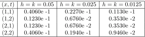
wheref(x, t) is selected such that the exact solution to bey(x, t) =cos(x+t). In this example, we obtain the results of Table 1. To compare, we report the results of [15] in Table 2.
Table 1. Absolute errors of Example5.1.
(x, t) h=k= 0.05 h=k= 0.025 h=k= 0.0125 (1,1) 0.2337e -4 0.4858e -5 0.1198e -7 (1,2) 0.1568e -4 0.1373e -5 0.5574e -7 (2,1) 0.1568e -4 0.1373e -5 0.5574e -7 (2,2) 0.2106e -3 0.1797e -4 0.2095e -5
Table 2. Results of [15] with Eulers method for Example5.1.
(x, t) h=k= 0.05 h=k= 0.025 h=k= 0.0125 (1,1) 0.4060e -1 0.2270e -1 0.1130e -1 (1,2) 0.1230e -1 0.6760e -2 0.3530e -2 (2,1) 0.1230e -1 0.6760e -2 0.3530e -2 (2,2) 0.4060e -1 0.1940e -1 0.9460e -2
Example 5.2. Consider the following two-dimensional VIE for (x, t)∈[0,1]×[0,1]
Zt
0 Z x
0
(xz2+cos(s))y(z, s)dzds=1 4x
5
−1 4x
5
cos(t) +1 4x
2
sin2(t),
with exact solutiony(x, t) =xsin(t). Table 3 shows the numerical result for this example withh=k= 0.01.
Table 3. Computational results of Example5.2forh=k= 0.01.
Example 5.3. Consider the third example in the form
Zt
0 Z x
0
(sin(tz) + 1)y(z, s)dzds=x
2
t2+ 2sin(xt)−2xtcos(xt)
2t2 sin(t),
(x, t)∈[0,1]×[0,1],
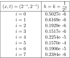
whose exact solution isy(x, t) = xcos(t). Table 4 shows the absolute errors at the points (x, t) = (2−i,2−i) fori= 0,1, ...,7.
Table 4. Computational results of Example5.3 forh, k= 1
27 at the points (x, t) = (2−i,2−i).
(x, t) = (2−i,2−i) h=k= 1
27
i= 0 0.5027e -6
i= 1 0.6169e -6
i= 2 0.1929e -6
i= 3 0.1517e -6
i= 4 0.2254e -5
i= 5 0.1570e -4
i= 6 0.1906e -5
i= 7 0.2384e -6
Example 5.4. Consider the following 2D-NVIEs
Zt
0 Z x
0
6 1 +z+su
3
(z, s)dzds= 2xt3+1 2(6x
2
+ 12x)t2+ 2x3t+ 6x2t+ 6xt,
(x, t)∈[0,1]×[0,1].
which has the exact solution as u(x, t) = x+t+ 1. To solve this equation, we substitute y(x, t) =u3(x, t) to get a linear equation.
Zt
0 Z x
0
6
1 +z+sy(z, s)dzds= 2xt
3
+1 2(6x
2
+ 12x)t2+ 2x3t+ 6x2t+ 6xt,
(x, t)∈[0,1]×[0,1].
Then we apply the method presented in this paper to obtain the results of Table 5. According to this Table, we see that the results improve when the step-lengthhandkdecrease.
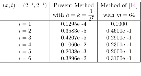
Example 5.5. Finally, let us consider [14]:
Zt
0 Z x
0
2ex+tu3(z, s)dzds=1 9(e
x+t−
e4x+t−ex+7t+e4x+7t),
(x, t)∈[0,1]×[0,1].
The exact solution isu(x, t) =ex+2t. Similar to the previous example, we substitutey(x, t) = u3(x, t) to get a linear equation.
Table 6 shows the absolute errors at some points using the presented method together with the results obtained by the method of [14] .
Table 5. Computational results of Example5.4for different values ofh, k.
(x, t) h=k= 0.05 h=k= 0.01 (0.1,0.1) 0.3715e -2 0.5400e -6 (0.2,0.3) 0.4380e -3 0.4086e -6 (0.4,0.7) 0.1592e -3 0.9868e -6 (0.5,0.5) 0.7246e -6 0.5612e -6 (0.6,0.3) 0.1084e -3 0.5864e -6 (0.8,0.8) 0.1019e -5 0.7435e -6 (1,0.9) 0.6840e -6 0.2859e -6
Table 6. Computational results of Example5.5.
(x, t) = (2−i,2−i) Present Method Method of [14]
withh=k= 1
27 withm= 64
i= 1 0.1295e -4 0.1000
i= 2 0.3583e -5 0.4600e -1
i= 3 0.4207e -5 0.2900e -1
i= 4 0.1060e -2 0.2300e -1
i= 5 0.2038e -3 0.2000e -1
i= 6 0.3896e -2 0.3100e -1
6. Conclusion
In this paper, we extended multi-step methods to solve two-dimensional nonlinear Volterra integral equations (2D-NVIEs) of the first kind. We converted a 2D-NVIE of the first kind to a one-dimensional VIE of the first kind and then we solved the resulted equations by using multi-step methods. The numerical results confirm the convergence and stability of the method. It seems that the presented method can be applied to other equations such as integro-differential equations.
Acknowledgment
The authors would like to thank Prof. S. Shahmorad for his thorough reviewing and valuable comments that helped the authors to improve the paper.
References
[1] G. A. Afroozi, J. Vahidi and M. Saeidy,Solving a class of two-dimensional linear and nonlinear Volterra integral equations by means of the Homotopy analysis method., I. J. Non. Sci,9(2010), 213–219.
[2] C. Andrade and S. McKee,On optimal high accuracy linear multistep methods for first kind Volterra integral equations., BIT Numer. Math,19(1979), 1–11.
[3] B. A. Beltyukov and L. N. Kuznechichina, A Runge-Kutta method for the solution of two-dimensional nonlinear Volterra integral equations., Diff. Eq.,12(1976), 1169–1173.
[5] W. A. Essah and L. M. Delves,The numerical solution of first kind integral equations., J. of Comput. and App. Math,27(1989), 363–387.
[6] S. Fazeli, G. Hojjati and H. Kheiri, A piecewise approximation for linear two-dimensional Volterra integral equations by Chebyshev polynomials., I. J. Non. Sci,16(2013), 225–261. [7] E. Goursat,Cours analyse mathematique., Vol. III, 5th ed. Paris: Gauthier-Villars (1942). [8] T. H. Gronwall,An integral equation of the Volterra type., Annals Math,16(1915), 119–122. [9] W. Holyhead, S. McKee and J. Taylor,Multistep methods for solving linear Volterra integral
equations of the first kind., SINUM,12(1975), 698–711.
[10] W. Holyhead and S. McKee,Stability and convergence of multistep methods for linear Volterra integral equations of the first kind., SINUM,13(1976), 269–292.
[11] A. Jerri,Numerical solution of some nonlinear Volterra integral equations of the first kind., John Wiley Sons, (1999).
[12] B. A. Lewis,On the numerical solution of Fredholm integral equations of the first kind., J. Inst. Math. and its App,16(1973), 207–220.
[13] E. Lin and Y. Al-Jarrah, Wavelet based methods for numerical solution of two-dimensional integral equations., Math. Aeterna,4(2014), 839–853.
[14] K. Maleknejad, S. Sohrabi and B. Baranji,Application of 2D-BPFs to nonlinear integral equa-tions commun., Nonlinear Sci. Numer. Simulat,15(2010), 725–735.
[15] S. Mckee, T. Tang and T. Diogo,An Euler-type method for two-dimensional Volterra integral equations of the first kind., Ima J. Numer. Anal,20(2000), 423–440.
[16] B. G. Pachpatte, Multidimensional integral equations and inequalities., ATLANTIS PRESS (2011).
[17] A. Tari and S. Shahmorad,Numerical solution of a class of two-dimensional nonlinear Volterra integral equations of the first kind., J. Appl. Math. & Inf,30(2012), 463–475.