Global Criterion Method Based on Principal Components to the Optimization of Manufacturing Processes with Multiple Responses

Global Criterion Method Based on Principal Components to the

Optimization of Manufacturing Processes with Multiple Responses

Gomes, J.H.F. – Salgado Jr., A.R. – Paiva, A.P. – Ferreira, J.R. – Costa, S.C. –Balestrassi, P.P. José Henrique de Freitas Gomes – Aluizio Ramos Salgado Júnior – Anderson Paulo de Paiva –

João Roberto Ferreira – Sebastião Carlos da Costa – Pedro Paulo Balestrassi*

Federal University at Itajuba, Institute of Production Engineering and Management, Brazil

The necessity of efficient and controlled processes has increased the demand by employing optimization methods to the most diverse industrial processes. For these cases, the Global Criterion Method is described in literature as a technique indicated for multi-objective optimizations. However, if the problem presents correlations between the responses, this technique does not consider such information. In this context, the Principal Component Analysis is a multivariate tool that can be used to represent correlated responses by uncorrelated components. Given that to negligence the correlation structure between the responses increases the likelihood of the optimization method in finding an inappropriate optimum point, the objective of this work is to combine the GCM and PCA in a strategy able to deal with problems having multiple correlated responses. For this reason, such strategy was used to optimize the 12L14 free machining steel turning process, characterized as an important machining operation. The optimized responses included the mean roughness, total roughness, cutting time and material removal rate. As input parameters, the cutting speed, feed rate and depth of cut were considered. Response Surface Methodology was employed to build the objective functions. The GCM based on principal components was successfully applied, presenting better practical results and a more appropriate location of the optimal point in comparison to the conventional GCM.

Keywords: multi-objective optimization, global criterion method, principal component analysis, free machining steel turning

0 INTRODUCTION

In industrial environments, it is becoming more and more important that items can be produced to satisfy several requirements simultaneously, and many of them are related to its cost, quality and productivity. Thus, considering that the manufacturing processes must be configured to obtain the best results for a set of characteristics, the interest in employing multi-objective optimization techniques has been increasing [1] and [2].

Among the optimization methods contemplating multiple responses, the desirability function [3], the multivariate integration [4] and the capacity indexes MCpm and MCpk [5] and [6] are listed as examples. Rao [7] describes the Global Criterion Method (GCM) as an interesting strategy. According to the author, the multiple objectives are optimized at the same time when the individual objective functions are combined in only one function, defined as the global optimization criterion of the process.

However, if the problem presents multiple correlated characteristics, the Global Criterion Method, as well as other conventional techniques, does not consider the correlation structure between the responses. This negligence, according to some researchers, may conduct the results to inadequate optimum points [8] and [9]. Paiva et al. [10] argue that the transfer functions used to represent the process outputs are strongly influenced by significant correlations existing between the responses of interest. Therefore, considering that the mathematical models

are of great importance to the problem formulation, non-consideration of the correlation structure will affect the optimal point location.

In attempt to offer a more adequate treatment to the optimization problems with multiple correlated responses, the Principal Component Analysis (PCA) has been shown as a good alternative [11] and [12]. The PCA consists in a multivariate statistical tool that concerns in explaining the variance-covariance structure of a data set, using linear combinations of the original variables. Thus, the original correlated responses are represented by new uncorrelated variables, called principal components.

Given that the Global Criterion Method is presented as a technique to multi-objective optimizations but does not take into account the correlation structure between the responses, the objective of this work is to incorporate the PCA in the original formulation for GCM described by Rao [7], and verify how this analysis influences in determining the optimal solution. For this, such techniques were applied on the 12L14 free machining steel turning process, characterized as one important operation in the modern industry.

1 THEORETICAL FRAMEWORK 1.1 Response Surface Methodology (RSM)

According to Montgomery [13], RSM is a collection of mathematical and statistical techniques that are useful for the modeling and analysis of problems in which a response of interest is influenced by several variables and the objective is to optimize this response.

The second order polynomial developed for

a response surface that relates a given response y

with k input variables presents the following format

described by Eq. (1):

y _ix x x x

i k

i ii

i k

i ij

i j i j

= + + +

= = _<

∑ ∑ ∑∑

β₀ β β β

1 1

2 _{, (1)}

where y is the response of interest, xi are the input parameters, β0, βi, βii, βij are the coefficients to be

estimated, and k is the number of input parameters

considered.

To estimate the coefficients stated in Eq. (1), the Ordinary Least Squares is the typically used algorithm. After the model building, the ANOVA statistical procedure is usually employed to check its significance and its adjustment.

1.2 Global Criterion Method (GCM)

A multi-objective optimization problem is one that, considering inequality constraints, can be stated as Eq. (2):

Minimize Subject to :

f f f

g j

p

j

1 2

0 1 2

x x x

x

( ) ( )

( )

( )

, ,...,

, , ,....,m , (2)

where fi(x) are objective functions, and gj(x)

constraints.

However, under various circumstances, the multiple responses considered in a process present conflict of objectives, with individual optimization leading to different solution sets. For this kind of problem, Rao [7] characterizes the Global Criterion Method as a strategy where the optimal solution is found by minimizing a preselected global criterion,

F(x), such as the sum of the squares of the relative deviations of the individual objective functions from the feasible ideal solutions. The GCM formulation is given by:

Minimize

Subject to :

F T f

T

g j

i i i i

p

j

x x

x

( )

( )



   

( )

2

1

0, ==1 2, ,..., , m

(3)

where F(x) is the global criterion, Ti is the target defined for the ith _{objective, fi (x) are objective} functions, gj (x) are constraints, and p is number of objectives.

Thus, with targets defined for each response of interest, the multiple objectives are combined into an only function, which becomes the global optimization function for the process.

To obtain the optimal point from GCM formulation, several optimization algorithms can be applied. In this work, the Genetic Algorithm was used because it is considered an effective algorithm to global optimizations [14] and [15].

1.3 Principal Component Analysis (PCA)

Suppose that the objective functions f1(x), f2(x),...,

fp(x), presented in Eqs. (2) and (3), are correlated with values written in terms of a random vector

YT _{= [Y1, Y2,..., Yp]. Assuming that Σ is the}

variance-covariance matrix associated to this vector, then Σ

can be factorized in pairs of eigenvalues-eigenvectors (λi, ei),..., ≥ (λp, ep), where λ1 ≥ λ1 ≥ ... ≥ λp ≥ 0, such

as the ith _{uncorrelated linear combination may be}

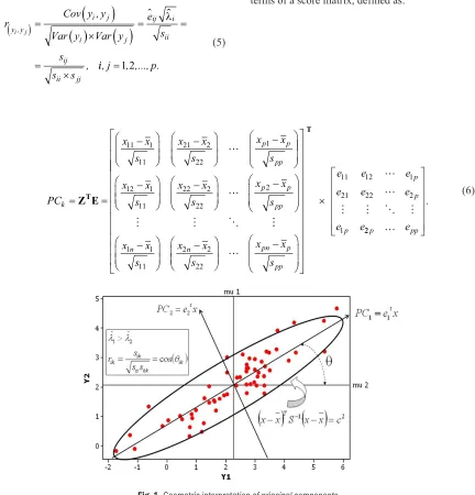
stated as PCi=eiTY=e Y e Y1 1i + 2 2i + +... e Ypi p, with i = 1, 2, ..., p. The ith _{principal component can be} obtained as maximization of this linear combination [16]. This statistical technique is called Principal Component Analysis (PCA), one of the most widely applied tools to summarize common patterns of variation among variables retaining meaningful information in the early PCA axes [17] and [18]. The geometric interpretation of these axes is shown in Fig. 1.

Generally, as the parameters ∑ eρ are unknown,

the sample correlation matrix Rij and the sample

variance-covariance matrix Sij may be used [16]. If the variables studied are taken in the same system of units or if they are previously standardized, Sij is a more

appropriate choice. Otherwise, Rijmust be employed

in the factorization. The sample variance-covariance matrix can be written as follows:

S

s s s

s s s

s s s

ij

p

p p pp

= 

    

11 12 1

21 22 21

1 2





     

=

(

)

(

)

(

)

= =

∑ ∑

,

s_ii 1 2, 1

1 1

n j y yi i s n y y y y

n

ij i i j j

j n

.

Then, the elements of sample correlation matrix

Rij can be obtained as:

r Cov y y

Var y Var y e s y y i j i j ij i ii

i j,

,

(

)

_{( )}

(

)

_{( )}

s s ,

ij

ii jj

ii j, =1 2, ,..., .p

(5)

In practical terms, the principal component (PC) is an uncorrelated linear combination expressed in terms of a score matrix, defined as:

PC x x s x x s x x s k p p pp = = −         −         −      

Z ET

11 1 11 21 2 22 1 _ −         −         −         x x s x x s x x s p p pp 12 1 11 22 2 22 2 x x s x x s x x s

n n pn p

pp 1 1 11 2 2 22 −         −         −                                     × T

e e e

e e e

e e

p

p

p

11 12 1

21 22 2

1

22p … epp              

. (6)

Fig. 1. Geometric interpretation of principal components

1.4 Global Criterion Method Based on Principal Components

The global criterion F(x), as stated by Eq. (3), is formulated from the objective functions and the targets defined to each response of interest. If the objective functions are unknown, then they can be modeled by RSM from experimental data. However, when the responses are correlated, this strategy does not take into account the correlation structure between them.

On the other hand, it has been seen in previous section that the principal components are characterized as uncorrelated representations of original correlated variables.

Minimize

Subject to :

F PC

g

PC PCi i

PCi i

k

j

x x

( )

( )



    =

∑ ζ ζ

2

1

xx

( )

j m

(7)

where FPC(x) is the global criterion based on

principal components, ζPCi is the target defined for the ith _{principal component, PCi(x) are quadratic} models developed for the principal components,

gj(x) are constraints, and k is the number of principal components considered.

The determination of the targets for principal components requires that the targets for original

responses are previously defined. The ζPCi is then

calculated as a linear combination between the eigenvectors of principal components and the standardized original responses in relation to their targets. This procedure is showed by Eqs. (8) and (9).

ζ_{PCi ji j} ζ_y

j p

e Z y _j

= ⋅

(

)

= ∑

1 , (8)

where ζPCi is the target defined for the ith _principal

component, p is the number of objectives, eji are

coefficients of the principal components’ eigenvectors, and Z(yj | ζyj) are the standardized original responses in relation to their targets, calculated as:

Z y_{j y} y yj

y j

j

j

ζ ζ

(

)

σ , (9)

where ζ_yj are targets defined for the original

responses, y_j are the means of responses, and σy_j

are the standard deviations of responses.

Analogously to the Eq. (3), the obtaining of optimal point for the formulation given in Eq. (7) is done by employing optimization algorithms. The Genetic Algorithm was also used in this work for this purpose.

Finally, for the Global Criterion Method based on principal components, it is important to highlight that this strategy combines the main advantages offered by GCM and ACP, since it continues being a technique for multi-objective optimizations, but now considering the correlation structure existing between the responses.

2 OPTIMIZATION OF THE 12L14 FREE MACHINING STEEL TURNING

With the aim of verifying the functionality of the GCM based on principal components in improving

performance of manufacturing processes, such strategy was applied to the optimization of 12L14 free machining steel turning process.

This is described as a relevant operation within the current industrial context, since the free machining steels are developed to offer good machining conditions and excellent chip formations. For this process, other mechanical characteristics, as ductility, strength and response to heat treatments are considered as secondary factors. The free machining steels have been employed in production of elements that do not need to present structural responsibility, as appliances and components to pumps, plugs and connections.

Due to the fact that mechanical properties are not the most important requirements for the 12L14 free machining steel turning process, its optimization is mainly concerned with its productivity and surface quality. The surface quality was then optimized

through the mean roughness (Ra) and total roughness

(Rt). For the productivity, cutting time (Ct) and

material removal rate (MRR) were the optimized

characteristics. The cutting speed (V), feed rate (f) and depth of cut (d) were considered as input parameters.

Given that the objective functions between the input parameters and responses were initially unknown, such relationships were modeled using RSM. Thus, data were collected from turning experiments performed with work pieces of 12L14 free machining steel (0.09% C; 0.03% Si; 1.24% Mn; 0.046% P; 0.273% S; 0.15% Cr; 0.08% Ni; 0.26% Cu; 0.001% Al; 0.02% Mo; 0.28% Pb; 0.0079%

N2), with dimensions of f40×295 mm. The machine

tool used was a NARDINI CNC lathe, with 7.5 cv power and maximum rotation of 4,000 rpm. The hard metal inserts (ISO P35 code SNMG 090304 – PM, Sandvik class GC 4035) were coated with three layers (Ti(C.N), Al2O3, TiN) and a tool holder ISO code DSBNL 1616H09 was employed.

3 RESULTS AND DISCUSSION 3.1 Modeling of Objective Functions

Writing the response surface function stated in Eq. (1) for three parameters, the following expression is obtained:

y V f d V f

d Vf Vd fd

= + + + + + +

+ + + +

β β β β β β

β β β β

0 1 2 3 11 2 22 2

33 2 12 13 23

.. (10)

To estimate the coefficients defined in Eq. (10),

the statistical software Minitab® was employed and,

from the experimental data presented in Table 2, the full quadratic models were developed for each response of interest. Then, the significance of models was tested through ANOVA procedure. Table 3 presents the coefficients for full quadratic models and the main results of ANOVA.

From Table 3 it can be observed that, considering a significance level of 95%, all models are adequate,

since p-values were lower than 0.05. Furthermore,

the adj. R2 _{values indicate high adjustments for the} models, which means these expressions are reliable in representing the responses.

Finally, after non significant coefficients have been removed, the final models, or the objective functions for responses, were obtained. Eqs. (11) to (14) present these expressions.

Ra V f d

V f d

= + + + −

− − − −

2 272 0 077 0 018 0 212 0 107 2 0 157 2 0 106 2 0 1

. . . .

. . . . 223fd , (11)

Rt V f d

f d Vf

= + − +

− − + −

12 708 0 172 0 254 1 418 0 643 2 0 511 2 0 302 0 5

. . . .

. . . . 118fd , (12)

Ct V f V

f Vf

= − − +

+ +

1 325 0 315 0 277 0 070

0 047 0 062

2 2

. . . .

. . , (13)

MRR V f d

Vf Vd fd

= + + + +

+ + +

26 600 5 679 5 082 6 997 1 140 1 500 1 400

. . . .

. . . . (14)

Table 1.Parameters and their levels

Parameter Symbol Unit Levels

-1.682 -1 0 +1 +1.682

Cutting speed V [m/min] 180 220 280 340 380

Feed rate f [mm/rev] 0.07 0.08 0.10 0.12 0.13

Depth of cut d [mm] 0.53 0.70 0.95 1.20 1.37

Table 2. Experimental matrix

Test Parameters Responses

V [m/min] F [mm/rev] d [mm] Ra [mm] Rt [mm] Ct [min] MRR [cm3_/min]

1 220 0.08 0.70 1.36 9.49 2.11 12.32

2 340 0.08 0.70 1.65 10.70 1.36 19.04

3 220 0.12 0.70 1.78 10.08 1.40 18.48

4 340 0.12 0.70 1.84 10.41 0.91 28.56

5 220 0.08 1.20 2.22 14.71 2.11 21.12

6 340 0.08 1.20 2.20 13.47 1.36 32.64

7 220 0.12 1.20 1.82 11.13 1.40 31.68

8 340 0.12 1.20 2.24 13.20 0.91 48.96

9 180 0.10 0.95 1.90 12.51 2.06 17.10

10 380 0.10 0.95 2.08 12.49 0.98 36.10

11 280 0.07 0.95 1.85 10.73 1.89 18.62

12 280 0.13 0.95 1.85 10.78 1.02 34.58

13 280 0.10 0.53 1.68 8.89 1.32 14.84

14 280 0.10 1.37 2.30 13.37 1.32 38.36

15 280 0.10 0.95 2.32 12.57 1.32 26.60

16 280 0.10 0.95 2.23 12.84 1.32 26.60

Table 3. Estimated coefficients for full quadratic models

Coeff. Responses

Ra Rt Ct MRR

β0 2.272 12.757 1.324 26.600

β1 0.077 0.172 -0.315 5.679

β2 0.018 -0.254 -0.277 5.082

β3 0.212 1.418 0.000 6.997

β11 -0.107 -0.038 0.070 0.000

β22 -0.157 -0.655 0.048 0.000

β33 -0.106 -0.522 0.002 0.000

β12 0.026 0.301 0.062 1.140

β13 0.006 -0.090 0.000 1.500

β23 -0.123 -0.518 0.000 1.400 p-value 0.002 0.005 0.000 0.000 adj. R2 _{[%] 85.46 80.63 99.68 99.72}

3.2 Optimization by Conventional Global Criterion Method

Before applying the GCM based on principal components to the optimization of 12L14 free machining steel turning, this operation was also optimized by conventional GCM, with the aim of comparing both results.

By taking the objective functions developed for the process responses, the GCM formulation can be built. However, for this formulation, it is necessary that the targets of original responses are defined. These specifications were made by experts and took into account that the process application could be satisfied with good levels of surface quality and productivity. Table 4 show the targets defined for responses and their respective specification limits.

Thus, the optimization problem was built as stated in Eqs. (15) to (17). All characteristics were considered with the same degree of importance.

MinG Ra Rt

Ct

= −



 



 + − 

 

  +

+ −



 

  + 1 5

1 5

9 0 9 0 1 2

1 2

3

2 2

2

. .

. . .

.

55 35

2

−  

 

 

MRR , (15)

subject to: V, f, d ≥–1.682 , (16)

V, f, d ≤1.682 , (17)

where G is the global criterion, Ra, Rt, Ct, MRR

are objective functions, and V, f, d are the input parameters.

Finally, replacing Ra, Rt, Ct and MRR in Eq. (15) by their respective objective functions, the final formulation of the problem was obtained given by:

MinG {[ ( V f

d V f

= − + + +

+ − − −

1 5 2 272 0 077 0 018 0 212 0 107 2 0 157 2 0

. . . .

. . . .1106

0 123 1 5 9 0 12 708 0 172

0 254 1 418

2 2

d

fd V

f d

−

− + − +

− +

. . . . .

. .

)] / } {[ (

−− − +

+ − + −

−

0 643 0 511

0 302 0 518 9 0 1 2

1 325 0

2 2

2

. .

. . . .

.

f d

Vf fd)] / } {[

-( .. . .

. . / .

.

315 0 277 0 070

0 047 0 062 1 2 35

26 6

2

2 2

V f V

f Vf

− + +

+ + + −

−

)] } {[

( 000 5 679 5 082 6 997

1 140 1 500 1 400 35 2

+ + + +

+ + +

. . .

. . . / ,

V f d

Vf Vd fd) ]}

(18)

subject to: V, f, d ≥–1.682 , (19)

V, f, d ≤1.682 . (20)

Table 4. Targets and specification limits for responses

Response LSL T USL

Ra 1.0 1.5 2.0

Rt 8.0 9.0 10.0

Ct 1.0 1.2 1.4

MRR 30 35 40

As can be observed, all optimized responses were established within the specification limits and relatively close to their targets, which suggests that it seems a good solution.

Table 5.Parameters used in Genetic Algorithm

Parameters Values

Iterations 1,000

Convergence 0.0001 Population size 150 Mutation rate 0.10

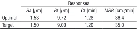
Table 6. Optimal results for 12L14 free machining steel turning obtained by conventional GCM

Responses

Ra [µm] Rt [µm] Ct [min] MRR [cm3_/min] Optimal 1.53 9.72 1.28 36.4 Target 1.50 9.00 1.20 35.0

The optimal point was found by applying Genetic

Algorithm in the previous formulation. Microsoft

Excel® was used for the mathematical programming

of problem and the Solver Evolutionary supplement

obtained with a cutting speed of 218 m/min, feed rate of 0.13 mm/rev and depth of cut of 1.24 mm.

3.3 Optimization by Global Criterion Method Based on Principal Components

Table 7 presents the correlation structure for Ra,

Rt, Ct and MRR. Since significant correlations were identified (p-value less than 0.05), the application of GCM based on principal components as optimization strategy is justified.

Table 7. Correlation structure of the responses

Ra Rt Ct

Rt 0.876

0.000

Ct –0.283 0.030 0.272 0.909

MRR 0.613 0.506 –0.701 0.009 0.038 0.002 Cells: Pearson correlation

p-value

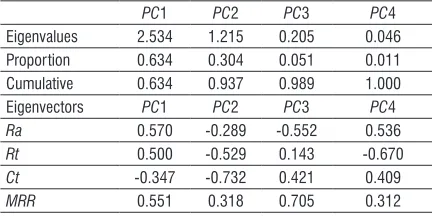
Table 8. Principal Component Analysis

PC1 PC2 PC3 PC4

Eigenvalues 2.534 1.215 0.205 0.046 Proportion 0.634 0.304 0.051 0.011 Cumulative 0.634 0.937 0.989 1.000 Eigenvectors PC1 PC2 PC3 PC4 Ra 0.570 -0.289 -0.552 0.536 Rt 0.500 -0.529 0.143 -0.670 Ct -0.347 -0.732 0.421 0.409 MRR 0.551 0.318 0.705 0.312

Performing the Principal Component Analysis for these responses (Table 8), it can be noticed that 93.7% of data are represented by two principal components. So, these new uncorrelated variables were used to substitute the original correlated responses.

Then, the objective functions for principal components were modeled taking the scores of each component obtained in the PCA. For this, the same procedure described in section 3.1 was employed.

Eqs. (21) and (22) present such functions for PC1

and PC2, which showed adj. R2 _{values of 94.18 and}

92.81%, respectively.

PC V f d

V f d

1 0 991 0 808 0 491 1 265

0 291 0 564 0 379

0

2 2 2

= + + + −

− − − +

+

. . . .

. . .

..156Vf −0 331. fd,

(21)

PC V f

d f d

Vf

2 0 457 0 633 0 742 0 452 0 289 0 279 0 202

2 2

= − + + −

− + + −

− +

. . .

. . .

. 00 342. fd.

(22)

Through Eqs. (8) and (9), the PC’s targets were calculated using data in Table 9. It resulted in values of -1.153 for PC1 and 2.077 for PC2.

Table 9. Used data to calculate the targets for principal components

Ra Rt Ct MRR

Mean 1.974 11.781 1.419 26.600 Std. dev. 0.280 1.622 0.396 9.707 Target 1.5 9.0 1.2 35 Standardization -1.692 -1.715 -0.554 0.865 Eigenvectors Ra Rt Ct MRR PC1 0.570 0.500 -0.347 0.551 PC2 -0.289 -0.529 -0.732 0.318

Finally, the formulation for GCM based on principal components was built, showing the following format:

MinGPC =− ₋ −PC PC



 1 153_{1 153} 1_ + _2 077_{2 077}− 2_

2 2

. .

.

. , (23)

subject to: V, f, d ≥–1.682 , (24)

V, f, d ≤1.682 , (25)

where GPC is the global criterion based on principal

components, PC1 and PC2 are objective functions

for the principal components, and V, f, d are the input parameters.

Replacing PC1 and PC2 in Eq. (23) by their

objective functions, the final formulation is written as:

MinG {[ ( V

f d V

PC = − − + +

+ + − −

1 153 0 991 0 808 0 491 1 265 0 291 2 0 564

. . .

. . . . ff

d Vf fd

2 2

2

0 379 0 156 0 331

1 153 2 077 0 457

−

− + −

− + − −

. . .

. . .

)] /

/( )} {[ ( ++ +

+ − + + −

− +

0 633

0 742 0 452 0 289 0 279

0 202 0 342

2 2

.

. . . .

. .

V

f d f d

Vf fd)] //2 077_. }2 _,

(26)

subject to: V, f, d ≥–1.682 , (27)

in Table 10, obtained for a cutting speed of 212 m/ min, feed rate of 0.13 mm/rev and depth of cut of 1.33 mm.

Table 10. Optimal results for 12L14 free machining steel turning obtained by GCM based on principal components

Responses

Ra [µm] Rt [µm] Ct [min] MRR [cm3_/min] Optimal 1.40 9.38 1.33 38.0 Target 1.50 9.00 1.20 35.0

Again, all optimized responses were established within the specification limits and relatively close to their targets. However, the global solution obtained with GCM based on principal components presented better surface finishing (lower roughness) and higher material removal. Although cutting time was higher, this solution was characterized as a more appropriate optimal point in relation to one obtained with the conventional GCM. Furthermore, this new optimal point was calculated taking into account the correlations between the original responses.

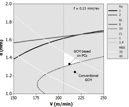
Fig. 2. Overlaid contour plot for the optimization of 12L14 free machining steel turning

Fig. 2 compares both optimal solutions with the feasible region for this problem. As easily noticed, the optimal point obtained with the conventional GCM, although seems a good solution, was established out of the feasible region. On the other hand, the solution found by GCM based on principal components, in addition to showing better practical results, was able to locate the optimal point inside the feasible region. The main argument for this fact is because the correlation structure of responses was considered in the second analysis. Thus, when correlations exist and are significant, the use of optimization strategies

that do not consider this information can conduct the problem to solutions that do not represent the best process condition.

4 CONCLUSIONS

This work presented the Global Criterion Method based on principal components as an alternative to optimize manufacturing processes with multiple correlated responses. From previous analysis, it was observed that the correlations are important information for this kind of problem and its negligence can direct the optimal point to inappropriate locations.

The GCM based on principal components was successfully applied to the optimization of 12L14 free machining steel turning process. An optimized condition with good surface finishing and good material removal was found for a cutting speed of 212 m/min, feed rate of 0.13 mm/rev and depth of cut of 1.33 mm. All optimized responses were established within the defined specification limits.

In comparison to the optimal point obtained with the conventional technique, the GCM based on principal components showed an optimal solution with better practical results in terms of roughness and material removal, but with a higher cutting time. In relation to the feasible region of the problem, the GCM based on principal components directed the optimal point to inside this region, while the solution found by conventional GCM stayed out of it. Due to these reasons, the optimal point found with GCM based on principal components was characterized as a more adequate solution.

Although the technique presented in this work has been effective to the optimization of 12L14 free machining steel turning, it needs to be tested in other processes. Therefore, it is suggested for future research works that this strategy is applied and verified in others turning applications and other manufacturing operations, like milling, cutting or welding.

5 ACKNOWLEDGEMENTS

The authors acknowledge the Capes, CNPq, FAPEMIG and the Institute of Mechanical Engineering of UNIFEI for supporting this work.

6 REFERENCES

[2] Župerl, U., Čuš, F. (2008). Machining process optimization by colony based cooperative search technique. Strojniški vestnik -Journal of Mechanical Engineering, vol. 54, no. 11, p. 751-758.

[3] Derringer, G., Suich, R. (1980). Simultaneous optimization of several response variables. Journal of Quality Technology, vol. 12, no. 4, p. 214-219.

[4] Chiao, H., Hamada, M. (2001). Analyzing experiments with correlated multiple responses. Journal of Quality Technology, vol. 33, no. 4. p. 451-465.

[5] Ch´ng, C.K., Quah, S.H., Low, H.C. (2005). Index Cpm in multiple response optimization. Quality Engineering, vol. 17, no. 1, p. 165-171, DOI:10.1081/ QEN-200029001.

[6] Plante, R.D. (2001). Process capability: a criterion for optimizing multiple response product and process design. IIE Transactions, vol. 33, no. 5, p. 497-509, DOI:10.1080/07408170108936849.

[7] Rao, S.S. (1996). Engineering optimization: theory and practice. 3rd _{ed. John Wiley & Sons, New Jersey.} [8] Khuri, A.I., Conlon, M. (1981). Simultaneous

optimization of multiple responses represented by polynomial regression functions. Technometrics, vol. 23, no. 4, p. 363-375, DOI:10.2307/1268226.

[9] Bratchell, N. (1989). Multivariate response surface modeling by Principal Components Analysis.

Journal of Chemometrics, vol. 3, no.4, p. 579-588, DOI:10.1002/cem.1180030406.

[10] Paiva, A.P., Paiva, E.J., Ferreira, J.R., Balestrassi, P.P., Costa, S.C. (2009). A multivariate mean square error optimization of AISI 52100 hardened steel turning. International Journal of Advanced

Manufacturing Technology, vol. 43, no. 7-8, p.

631-643, DOI:10.1007/s00170-008-1745-5.

[11] Wang, F.K., Du, T.C.T. (2000). Using Principal Component Analysis in process performance for multivariate data. Omega, vol. 28, no. 2, p. 185-194, DOI:10.1016/S0305-0483(99)00036-5.

[12] Rossi, F. (2001). Blending response surface methodology and principal components analysis to match a target product. Food Quality and

Preference, vol. 12, no. 5, p. 457-465, DOI:10.1016/

S0950-3293(01)00037-4.

[13] Montgomery, D.C. (2005). Design and Analysis of

Experiments. 6th _{ed.: John Wiley, New York..}

[14] Ficko, M., Brezocnik, M., Balic, J. (2005). A model for forming a flexible manufacturing system using

genetic algorithms. Strojniški vestnik - Journal of

Mechanical Engineering, vol. 51, no. 1, p. 28-40.

[15] Busacca, G.P., Marseguerra, M., Zio, E. (2001). Multiobjective optimization by Genetic Algorithms: Application to safety systems. Reliability

Engineering & System Safety, vol. 72, no. 1, p.

59-74, DOI:10.1016/S0951-8320(00)00109-5.

[16] Johnson, R.A., Wichern, D. (2002). Applied

Multivariate Statistical Analysis. 5th _ed.

Prentice-Hall, New Jersey.

[17] Ronggen, Y., Ren, M. (2011). Wavelet denoising using principal component analysis. Expert Systems

with Applications, vol. 38, no. 1, p. 1073-1076,

DOI:10.1016/j.eswa.2010.07.069.

[18] Ho, C.T.B., Wu, D.D. (2009). Online banking performance evaluation using data envelopment analysis and Principal Component Analysis.

Computers & Operations Research, vol. 36, no. 6, p.