Volume 8, Number 4, pp. 423–435.http://www.scpe.org 2007 SWPS
TIME QUANTUM GVT: A SCALABLE COMPUTATION OF THE GLOBAL VIRTUAL TIME IN PARALLEL DISCRETE EVENT SIMULATIONS
GILBERT G. CHEN∗ AND BOLESLAW K. SZYMANSKI†
Abstract. This paper presents a new Global Virtual Time (GVT) algorithm, called TQ-GVT that is at the heart of a new high performance Time Warp simulator designed for large-scale clusters. Starting with a survey of numerous existing GVT algorithms, the paper discusses how other GVT solutions, especially Mattern’s GVT algorithm, influenced the design of TQ-GVT, as well as how it avoided several types of overheads that arise in clusters executing parallel discrete simulations. The algorithm is presented in details, with a proof of its correctness. Its effectiveness is then verified by experimental results obtained on more than 1,000 processors for two applications, one synthetic workload and the other a spiking neuron network simulation.
Key words. global virtual time, time warp, parallel discrete event simulation, scalability
1. Introduction. Parallel discrete event simulators [1] are perhaps among the most sophisticated dis-tributed systems developed. A Parallel Discrete Event Simulation (PDES) must execute events according to their inherent timestamp order which may differ from the order in which they are created. Historically, two main methods have been introduced to deal with this problem, one called conservative [2, 3] and the other optimistic (or Time Warp) [4].
The notion of Global Virtual Time (or GVT) [4] was first introduced by Jefferson to track the earliest unprocessed events in the entire simulation. By definition, GVT at any given instance of the simulation execution is the minimum value among the local virtual times of all processors and the timestamps of all messages in transit. Any processed event with a timestamp earlier than the current GVT will not be rolled back under any circumstances, and therefore the memory associated with it can be safely released. Without the notion of GVT, the Time Warp mechanism would be impractical because of its huge memory consumption. However, it is impossible to compute the exact GVT as it would require collecting information on distributed processors at exactly the same wall-clock time. Fortunately, a lower bound on GVT is also useful as events earlier than such a bound can be safely removed. Although events with a timestamp larger than the GVT estimate but smaller than the true GVT value cannot be removed, those events should not have a significant impact on memory usage, as long as the GVT estimate is sufficiently close to the true GVT value.
GVT computation is perhaps the only global operation in Time Warp. All others, such as rollbacks, state saving, and sending and handling of anti-messages, can be carried out locally. Therefore, GVT computation is known to be the least scalable component of Time Warp and it is no surprise that the accuracy and overhead of the GVT computation may dominate the overall performance of Time Warp.
GVT is useful not for Time Warp only. A few variants of conservative protocols, such as the conditional event approach [5] and the LBTS approach [6], which largely depend on the amount of lookahead, also need to compute Lower Bound on Time Step (LBTS) which computationally is equivalent to GVT. In our future work, we will evaluate performance of TQ-GVT for such software platforms. The less-known third class of PDES protocols is based on lookback [7, 8] and some of its variants (see [9] for details) rely on prompt GVT estimates as well. A good GVT algorithm is the key to the efficiency of these protocols.
Numerous GVT algorithms [10]–[24] have been devised. Many papers introducing them [10, 11, 14, 16, 20, 22] focused on feasibility and correctness of GVT computation but did not provide performance data. Those that did, gave the results of runs with quite limited number of processors. The largest Time Warp simulation that has been described in the literature, in terms of the processor count, was presented in [25], which, however, did not employ a general GVT algorithm. The largest Time Warp simulation with a general GVT algorithm was reported in [26] with runs on 104 processors. The first Time Warp simulator, Time Warp Operating System, had to limit GVT computation frequency to less than one execution per every 5 seconds on 32 processors, because of its overhead [27].
This paper presents a new GVT algorithm, called Time Quantum GVT (TQ-GVT), which, although con-ceptually simple, is efficient and scalable. TQ-GVT has proven to be able to deliver GVT estimates every tenth of a second on as many as 1,024 processors. The associated overhead is small: each GVT message is either 16
∗Center for Pervasive Computing and Networking, RPI, Troy, NY, 12180, USA ([email protected]). †Department of Computer Science, RPI, Troy, NY, 12180, USA (
or 48 bytes long. In addition, the total number of GVT messages needed for each GVT computation is always twice the number of processors. Hence, the number of GVT messages per processor is constant, independent of the number of processors used. As a result, the aggregate network bandwidth consumed by GVT computation alone is less than 1 Mbytes per second on a parallel computer with 1,024 processors.
The paper first surveys other GVT algorithms. It then describes how TQ-GVT works, proves its correctness, and provides concrete evidence that TQ-GVT works as expected on two applications, one synthetic and the other realistic. Finally, it concludes by summarizing the properties of TQ-GVT and by outlining an additional research that can be done on this topic.
2. Related Work. Designs of GVT algorithms focus on either shared-memory or distributed computers. Shared-memory GVT algorithms assume that certain variables are accessible by all processors [28, 29], so they perform well on Symmetric Multi-Processing machines, but their performance is unclear on Non-Uniform Memory Access ones in which dependence on global variables limits scalability of any algorithm.
Distributed GVT algorithms do not use global variables and therefore are more scalable. By definition, GVT at a wall-clock time is either the smallest local virtual time or the smallest timestamp of all messages in transit. As it is impossible to measure local virtual times at the same wall-clock time on different processors, techniques were needed to make the measurements look like they were taken simultaneously. Most of these techniques are in general based on overlapping intervals [10, 12, 14, 16, 19], two cuts [13, 17], or global reduction [18, 20, 21].
Overlapping Intervals. The overlapping interval technique selects an interval of wall-clock time for each processor, such that the intersection of all intervals is nonempty. Any point in wall-clock time within this intersection can be viewed as an instant at which the GVT measurement was taken. The smallest local virtual time at any such instant is guaranteed to be no smaller than the smallest local virtual time within the intersection of all intervals.
Two methods are normally used for building these overlapping intervals. The first method, widely used in early GVT algorithms, consists of broadcasting two messages from an initiator [12, 14, 19], a START message to begin the process, and then, after receiving responses from all processors, a STOP message, after which the initiator waits for responses again. The times of receiving of START and STOP messages on each processor (and the last response on the initiator) define the interval. The second method of building overlapping intervals involves circulation of a special token between processors, normally in a predefined topology, and the interval starts with one arrival of the token, and ends with its next arrival [10].
However, the overlapping intervals technique presents only a partial solution. Another problem that needs to be addressed by GVT algorithms is how to account for transient messages, the second part of the GVT definition. Transient messages are those that have been sent but have not been yet received. They must be accounted for by either the sender processor or the receiver processor, or both. The simplest solution is to use message acknowledgments, so that any message whose acknowledgments has not been received is deemed to be transient and its timestamps must be included in the GVT computation.
It is no coincidence that earlier GVT algorithms [12, 14, 19] often implemented the message acknowledgment scheme, for it is a simple solution. However, its primary drawback is that it almost doubles the total number of messages sent in the simulation, so the performance may deteriorate. A natural optimization is not to use separate acknowledgment messages, but to piggy-back acknowledgments in normal messages that carry events [10]. Still, such an optimization does not completely alleviate the problem.
Lin and Lazowska [16] proposed to use sequence numbers to reduce acknowledgment overhead. Messages sent from one processor to another are marked with consecutive, increasing sequence numbers. When GVT related information is needed, processors will notify neighbors of the latest sequence numbers they have seen. These sequence numbers tell which messages have been received, and which have not.
Another drawback of the message acknowledgment scheme is quite subtle. It is not a trivial task to find out the earliest timestamp among unacknowledged messages. Such an operation is not of constant time and may require the use of a priority queue.
GVT can be computed from the local virtual times at cut points of a consistent cut and the set of transient messages (which are now defined as messages traveling from the past to the future).
Another, simpler solution, widely known as Mattern’s GVT algorithm, attempts to construct two cuts. Luckily, neither cut needs to be consistent. The only requirement is that all messages sent before the first cut must be received before the second cut. The GVT estimate is now the minimum of the local virtual times at the cut points on the second cut, or the smallest timestamp of the messages sent after the first cut, whichever is smaller. Messages crossing the second cut from the future to the past can be ignored, since these messages are guaranteed to have a timestamp larger than the GVT value.
In its original form, Mattern’s GVT algorithm uses token passing to construct the two cuts [17]. A vector clock, contained in the token being passed between processors, monitors the number of transient messages sent to every processor. The token can leave the current processor only after all messages destined to it have been received. Thus, the second cut can be built with only one round of token passing, but its creation may incur a delay on each processor.
Mattern proposed several variants to remove the vector clock or the delay on every processor [17]. In one, a scalar counter replaces the vector clock. However, now the second cut is not guaranteed to be done with one round of token passing; several rounds may be necessary. Mattern also presented another variant in which a single round is sufficient without the use of vector clock. However, it still requires tokens to be delayed on each processor.
Choes and Tropper [13] improved the original Mattern’s GVT algorithm by using a scalar counter to track the number of messages sent before the first cut. When this counter reaches zero, no more messages originating from before the first cut are in transit, which signals the completion of the second cut. Even though multiple rounds may be needed, the authors observed that two rounds are sufficient in most cases.
There are two other GVT algorithms which do not appear similar to Mattern’s GVT algorithm but in fact are based on the idea of constructing consistent cuts. In Tomlinson and Garg’s GVT algorithm [22], simulation times instead of wall-clock times are used to schedule GVT computations. A cut point is the point at which a processor reaches a scheduled simulation time, and extra consideration must be taken to ensure a consistent cut. Bauer and Sporrer’s GVT algorithm [11] identifies reports that form a consistent cut, and then uses these reports to derive a GVT estimate.
Global Reduction. Global Reduction is a simplification of Mattern’s GVT algorithm. When all processors arrive at a synchronization point, a global reduction is performed on the number of transient messages that were sent and not received before the synchronization point. When this number becomes zero, it is apparent that no transient messages exist so that the information collected at the synchronization point can be used to compute the GVT estimate.
Perumalla and Fujomoto [18] presented a global reduction GVT algorithm which divides the time lines into bands. Bands are constructed in such a way that the messages sent during one band are guaranteed to be received in the current or next band. Thus, the boundaries of a band form two consecutive cuts, as in Mattern’s GVT algorithm.
Steinman et al [21] described a synchronous GVT algorithm also based on global reduction. Srinivasan and Reynolds [20] developed yet another GVT algorithm that relies upon global reduction, but their algorithm requires hardware support.
Other Algorithms. There are some GVT algorithms that cannot be easily grouped into any of the three categories discussed so far. The pGVT algorithm [15] uses a GVT manager to monitor the progress of every processor and to compute the GVT based on information collected from processors. Processors are required to report to the GVT manager whenever they receive a straggler message. The Seven O’clock algorithm [23] assumes that the underlying network can always deliver events within a certain time window. Based on this assumption, a new notion called Network Atomic Operation is introduced which then extends Fujimoto and Hybinette’s shared-memory GVT algorithm [28] to the distributed memory domain. A similar idea that enables bypassing message acknowledgment if the maximum transmission delay is known has been introduced in [14].
Table 2.1
Comparison of Various GVT Algorithms
Authors Idea Ack Vector Channel Scalability
Samadi [19] Broadcast START and
STOP messages to form overlapping intervals
Yes No Any N/A
Bellenot [12] Use message routing graph
instead of broadcast
Yes No Any 104 [26]
Das and Sarkar [14] Optimize the computation
for hypercube topology
No No Maximum
Delay N/A
Baldwin, Chung and
Chung [10]
Pass a token to form overlapping intervals
Yes No FCFS N/A
Lin and Lazowska
[16] Send valley messages to
reduce acknowledgement traffic
Implicit No Any N/A
Mattern [17] Construct two cuts such that
no transient messages sent before the first cut exist
No Yes Any 12 [13]
Choe and Tropper
[13] Create multiple rounds of token passing to form the
two cuts
No No Any 12 [13]
Tomlinson and Garg
[22] Build consistent cuts by
using TGVT events
No Yes Any N/A
Bauer and Sporrer
[11] Identify pairs of reports that form a consistent cut No No FCFS N/A
Srinivasan and
Reynolds [20] Use hardware-based global reduction No No Any N/A
Steinman, Lee, Wilson, and Nicol
[21]
Use global reduction No No Any 64 [21]
Perumalla and
Fujimoto [18] Use global reduction No No Any 16
[18]
D’Souza, Fan, and
Wilsey [15] Report stragglers to a GVT manager Yes No Any 2
[15]
Bauer, Yuan, Carothers, Yuksel, and Kalyanaraman
[23]
Extend Fujimoto’s shared-memory GVT algorithm with the notion of network atomic operations
No No Maximum
Delay
16 [23]
Deelman and Szymanski [24]
Use vector and matrix clocks to keep track of messages in transit
No Yes Any 16 [24]
disadvantage of this algorithm is the need of communicating a matrix of processor knowledge about messages in transit that is of the rank of the number of direct outgoing connections. Hence, this algorithm is scalable only in applications in which the out-degree of all nodes in the processor communication graph is independent of the graph size.
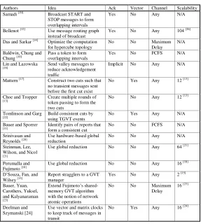
Summary of Existing GVT Algorithms. Table 1 summarizes the key ideas behind various GVT algorithms and their requirements, such as the need of acknowledgments, the use of vector clocks, and the type of the communication channels required. It also lists the highest number of processors on which each of them has been run and reported in the literature.
When considering requirements for a highly scalable GVT algorithm, we identified several properties that should be avoided as they limit scalability. First of those is the need for message acknowledgments that increase the network traffic and interfere with the transmission of normal messages. Lin and Lazowska’s idea [16] eliminates the necessity of explicit acknowledgments, but at the expense of larger latency of GVT computation and of complex data structures to store messages. Second such property is the use of any vector whose size is linear with the number of processors. Finally, a truly scalable algorithm should not impose any special requirements on the communication channel except two basic ones, the First-Come-First-Served order of delivery and reliable (no-loss) delivery. These two requirements are satisfied by many popular communication libraries, such as MPI or TCP/IP.
problem is that they all attempt to determine the completion of the second cut collectively by all processors. Motivated by this analysis, we propose an alternative, which constructs the second cut in a centralized way, thus avoiding the scalability problems that may arise when these approaches are used on a very large number of processors.
3. Overview of Time Quantum GVT. Two essential features distinguish Time Quantum GVT (TQ-GVT) from other GVT algorithms. First, TQ-GVT assigns the task of GVT computation to one processor, which is then referred to as the GVT master. The GVT master does not perform any simulation; its responsi-bilities include only collecting GVT reports, as well as calculating and distributing GVT. All other processors, called simulating processors, on the other hand, are not directly involved in the GVT computation. This ap-proach is basically a centralized one; however, it differs from other centralized apap-proaches in that the GVT master never initiates GVT calculations. Instead, the GVT master passively listens to GVT messages and takes actions only when they come. In this respect, TQ-GVT is similar to the pGVT algorithm [15], which, however, requires that simulating processors report to a dedicated processor every time a straggler arrives.
Second, TQ-GVT divides the wall-clock time into a continuous sequence of time quanta with equal width. Time quanta need not be precisely synchronized on different processors. Each processor maintains a counter indicating the index of the current time quantum and increases the counter at the end of the time quantum defined by its own hardware clock. Every message is marked with the index of the time quantum from which it is sent. The purpose of time quantum is to group messages, so if there is a way to track the number of transient messages from each time quantum, then, in computing GVT, only time quanta with messages in transit need to be taken into account.
Time quanta are similar to bands described in [18] in which, however, the division of the wall-clock time into bands is driven by the completion of the corresponding GVT computation. As a result, in the algorithm proposed in [18], processors cannot proceed to the next band if the GVT computation has not finished. In contrast, in TQ-GVT, the results or status of GVT computation have no impact on the division of wall-clock into time quanta.
Processor 1
Processor 2
Processor 3
Processor 4
Time Quantum 0 1 2 3 4
Reports Completed Cuts
First Cut Second Cut
Wall-clock Time
Fig. 3.1.An Illustration of the Time Quantum GVT Algorithm
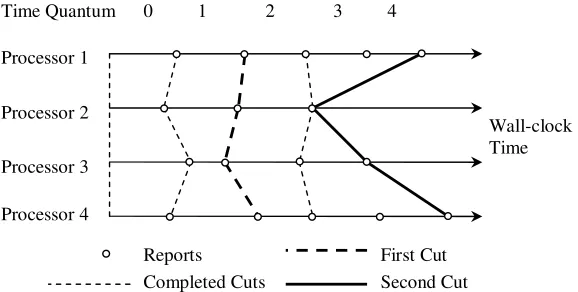
Figure 1 illustrates the basic idea of TQ-GVT. Small circles indicate the wall-clock times at which processors advance to next time quantum and send out GVT reports. The GVT master constructs cuts from the reports stamped with the same time quantum index. If, for a particular time quantum, the reports from all processor have been received, then the cut is regarded as completed. The GVT master monitors the number of sent as well as the number of received messages within each time quantum, based on information carried in the GVT reports. If the two numbers associated with a given time quantum are equal, then all messages sent during this time quantum must have already been received. Hence, the algorithm is based on the Mattern’s idea of two cut [17]: the first cut consists of reports for the latest time quantum that contains no transient messages, and the second cut consists of latest reports from every processor.
whether or not there are still messages in transit from each time quantum and calculates the GVT accordingly. Empirically, in current hardware platforms, one GVT master can drive as many as 128 simulating processors, so an extra level of intermediate masters is needed to increase the number of simulating processors to 16,384. If this is not sufficient, more levels of GVT masters can be added. A very small percentage of processors, 129 out of 16,513, or merely 0.78 percent, will not be directly participating in the simulation. Hence, such a solution is suitable for clusters in which the numbers of processors involved in a computation are large. It should be noted that the use of such reduction network for conservative parallel discrete simulation was introduced already (see [6]), however, the reduction was applied to all simulation processors, unlike in our solution in which only GVT masters participate in reduction.
Two factors contribute to the low overhead of TQ-GVT. First, in TQ-GVT, GVT computation does not interfere with other simulation activities. Simulating processors are only engaged in processing events and transmitting and receiving messages. To support GVT computation, they just need to send report messages periodically, and to receive GVT messages as they come. If GVT messages do not come on time, simulating processors are never delayed or blocked, as in the case of some other algorithms, unless the delay is so large that it begins to interfere with fossil collection. As a result, only the GVT masters are involved in a significant amount of GVT computation. Since this is their sole task, the GVT masters can respond to incoming messages more swiftly than simulating processors which would have to switch between checking and receiving incoming messages and processing events. The cost of GVT computation for simulating processors is a non-blocking send of a report message at the end of each quantum and a non-blocking receive of the new GVT value if there is a GVT message.
Second, in TQ-GVT, different rounds of GVT computation are overlapped. One round does not need to be completed before the next round starts. For example, a processor can keep sending the GVT master a report message at the end of each time quantum, even if the reports from previous quanta have not reached the GVT master yet. The GVT master decides which reports to use based on the number of transient messages in each time quantum. Thus, this solution is insensitive to the large latency of the interconnection network often found in clusters, as well as to the local clock asynchrony that results in different processors reaching the synchronization point at different wall-clock times.
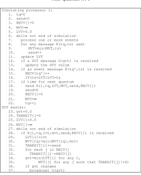
4. Detailed Description of TQ-GVT. TQ-GVT uses three types of messages. An event message, denoted byE(tq, ts), is the carrier of a positive event or an anti-event, wheretsis the timestamp andtqis the index of the time quantum from which the event was sent. A GVT messageG(gvt) simply contains the value of the new GVT estimate. A report message has the format ofR(i, tq, LV T, M V T, send, RECV[]), where iis the processor id, tq is the index of the current time quantum, LV T is the local virtual time,M V T is the earliest event sent during the current time quantum, send is the count of messages sent out during the current time quantum, andRECV[] is a vector of integers, each of which denotes the number of events received that were sent from the corresponding time quantum.
In Figure 2, lines 1-22 show the procedure executed on simulating processors and lines 23-37 the procedure of the GVT master. Lines 1-5 initialize variables needed by report messages. Lines 6-22 are the main loop of the simulation. Among them, lines 7-11 process one or more events and update MVT and LVT accordingly. Lines 12-13 check if a new GVT estimate is available. Lines 14-16 receive any incoming messages, and update RECV[] and LVT accordingly. Lines 17-22 send a new report to the GVT master, reset variables and then advance to next time quantum.
For GVT master, lines 23-26 initialize several variables needed to compute the GVT.T RAN SIT[] represents the number of transient event messages for every time quantum, LV T[] stores the local virtual time for each processor, and M V T[] stores the smallest timestamp sent during each time quantum. The main simulation loop keeps receiving report messages until the end of simulation. For every received report, at lines 29-33, the GVT master updates the corresponding elements inLV T[],M V T[], andT RAN SIT[]. At lines 34-35, the GVT master attempts to calculate a new GVT estimate as the minimum of the LVT of all processors and the MVT of all time quanta that still have event messages in transit. If the new GVT estimate is different from the old one, it will be broadcasted to every simulating processor.
Simulating processor i: 1. tq=0
2. send=0 3. RECV[]=0 4. MVT=∞ 5. LVT=0.0
6. while not end of simulation 7. process one or more events 8. for any message E(tq,ts) sent 9. MVT=min(MVT,ts)
10. send++ 11. update LVT
12. if a GVT message G(gvt) is received 13. update the GVT value
14. if an event message E(tq',ts) is received 15. RECV[tq']++
16. if(ts<LVT)LVT=ts 17. if time for next quantum
18. send R(i,tq,LVT,MVT,send,RECV[]) 19. send=0
20. RECV[]=0 21. MVT=∞ 22. tq++; GVT master:
23.gvt=0.0 24.TRANSIT[]=0 25.LVT[]=0.0 26.MVT[]=∞
27.while not end of simulation
28. if R(i,tq,lvt,mvt,send,RECV[]) is received 29. LVT[i]=lvt
30. MVT[tq]=min(MVT[tq],mvt) 31. TRANSIT[i]+=send
32. for each j in RECV[] 33. TRANSIT[j]-=RECV[j] 34. gvt=min(LVT[i] for any i,
35. MVT[j] for any j such that TRANSIT[j]!=0) 36. if gvt changes
37. broadcast G(gvt)
Fig. 4.1.TQ-GVT: Program for Simulating Processors and GVT Master
Hence, in the actual implementation, we use a maximum length k on this vector, so messages received from k oldest active time quanta are reported. By doing so, the correctness of the algorithm is not changed; the only effect may be that the GVT will be more conservatively computed. This happens because at most k time quanta can be removed from consideration at the end of each time quantum by the GVT master. In our limited experiments,k set to 2 or 4 gave the best performance. In summary, only a vector of size k with each entry containing a number of received messages in the corresponding time quantum needs to be sent to the GVT master, making the length of report messages constant, regardless of how many processors are being used.
The code for intermediate level GVT masters is not presented here. The reason is simple: these GVT masters act as messengers that merely forward any messages they receive. They may perform some optimization, such as combing multiple report messages coming from different processors but with the same time quantum index into a single report message. The only effect of using intermediate GVT masters is the prolonged communication delay. However, as evident in the next section, TQ-GVT does not impose any limitation on message transmission delay, so the discussion on intermediate GVT masters is omitted.
5. Correctness of TQ-GVT. To prove the correctness of a GVT algorithm, a usual approach is to show that neither the transient message problem nor the simultaneous reporting problem exists [16, 30]. Here, a different approach will be used. Instead of proving that what TQ-GVT computes is a lower bound estimate of the GVT value according to the authentic definition of GVT, we will prove the correctness of TQ-GVT based on a “utilitarian” definition of GVT (similar technique was used in [28] for a different GVT algorithm). That is, we will show that the following Lemma holds.
Lemma. If an event message m1 with timestamp ts(m1) is received after a GVT value gvt is received,
Proof. We prove this property by contradiction using induction. Hence, we assume that a processori1sent
at time quantum s1 a messagem1 such thatts(m1) < gvt. Let j1 be the time quantum from which the last
report message was sent by processori1and received by the GVT master before the currentgvtwas obtained.
LetLV Ti,j denote the local virtual time reported by processoriat the end of time quantumj.
It cannot be thatts(m1)≥LV Ti1,j1, sinceLV Ti1,j1 is taken into account in computinggvt, soLV Ti1,j1 ≥
gvt. Neither it could be thats1≤j1, since thents(m1) would be reflected in the MVT value corresponding to
s1, contradicting our assumption thatts(m1)< gvt. Hence, s1> j1 andts(m1)< LV Ti1,j1, so there must be
another messagem2, sent by a different processori2, which caused a rollback on processori1, and this message
timestamp satisfies the inequalitygvt > ts(m1)> ts(m2), as a rollback never affects the events with the same
or earlier timestamps than the timestamp of the rollback message itself. From that it follows that messagem2
also satisfiess2> j2, wheres2, j2 are analogs ofs1, j1.
By induction, let’s assume that there is a messagemk, sent by processor ik, such that ts(mk)< gvt and sk > jk, where jk denotes the latest time quantum on processorik that is included in the current value of gvt and sk is the time quantum at which messagemk was sent. It cannot be thatts(mk)≥ LV Tik,jk, since
LV Tik,jk is taken into account in computinggvt, soLV Tik,jk≥gvt. Hence,ts(mk)< LV Tik,jk, so there must
be another message mk+1, sent by a different processor ik+1, which caused a rollback on processor ik, and this message timestamp satisfies the inequality gvt > ts(mk)> ts(mk+1). We define sk+1, jk+1 as analogs of
sk, jk. For messagemk+1, it cannot be thatsk+1≤jk+1, since thents(mk+1) would be reflected in MVT value
corresponding tosk+1, contradicting our conclusion thatgvt > ts(mk+1).
Hence, by induction we conclude that our assumption that ts(m1)< gvtimplies that there is an infinite
sequence of messages with timestamps smaller thangvt, which contradicts the basic premise that each simulation can generate only a finite number of messages in the finite simulation timegvt.[]
The above proof makes no assumption on the delay of massage passing. Therefore, the use of intermediate GVT masters will not affect the correctness of TQ-GVT.
6. Experimental Results. TQ-GVT has been implemented in DSIM [31], a new distributed Time Warp simulator available freely at http://www.cs.rpi.edu/ cheng3/dsim. Although DSIM features several novel techniques that effectively reduce the overhead of Time Warp operations, we are convinced that TQ-GVT is the main thrust that enables DSIM to scale to at least 1,024 processors without any sign of loss of efficiency.
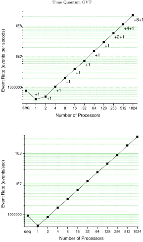
Two applications have been built on top of DSIM to test the scalability of the simulator, as well as of the new GVT algorithm. The first application is a simulation of the PHOLD benchmark, a synthetic workload generator proposed by Fujimoto [32]. In our version of the PHOLD benchmark, each event stays at an LP (Logical Process) for a time randomly chosen from the exponential distribution and then departs to one of four nearest neighbors randomly chosen. LPs are organized into a two dimensional grid. Strip partitioning is utilized, which allocates a continuous set of columns of LPs to the same processor. Although simple, the PHOLD model is difficult to parallelize for two reasons. First, there is no lookahead in it, so conservative protocols do not apply. Second, the event granularity is low, so the efficiency of parallelization is very sensitive to its overhead. All the experiments were run on the Lemieux cluster at Pittsburgh Supercomputing Center consisting of 750 nodes, each with 4 AlphaServer processors, connected by a Quadrics interconnection network. The top part of Figure 3 shows the committed event processing rates of DSIM running the PHOLD benchmark on up to 1024 processors for about 50 sec of simulation time. Each simulating processor simulated 8 columns of LPs, with 8,192 LPs in each column, regardless of the total number of processors used, so the workloads on each processor remained constant, while the size of grid increased linearly with the number of processors. A number associated with each data point indicates the number of extra processors allocated exclusively to executing the TQ-GVT algorithm. It was determined empirically that each GVT master can drive as many as 128 processors. Starting from 256 processors, an extra level of up to 8 intermediate GVT masters were introduced.
0.5 1 2 4 8 16 32 64 128 256 512 1024 1000000
1E7 1E8
+8+1
+4+1
+2+1
+1
+1
+1
+1
+1
+1
+1
E
v
e
n
t
R
a
te
(
e
v
e
n
ts
p
e
r
s
e
c
o
d
s
)
Number of Processors seq
+1
0.5 1 2 4 8 16 32 64 128 256 512 1024 1000000
1E7 1E8
E
v
e
n
t
R
a
te
(
e
v
e
n
ts
/s
e
c
)
Number of Processors seq
Fig. 6.1.Event Processing Rates with the PHOLD (top) and Spiking Neural Network (bottom)
case) interactions with the GVT master slowing the progress of a parallel processor. However, all these factors contribute a constant overhead per each parallel processor, so the parallel performance grows practically linearly with the number of parallel processors used.
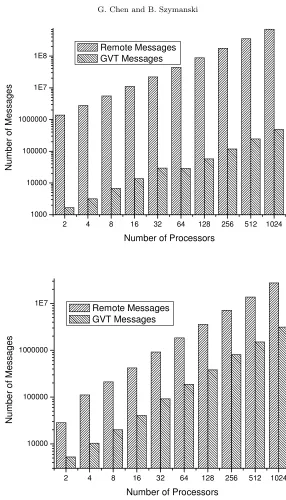
For the largest simulation with 1024 processors, over 11 billion committed events were processed, over 3 million rollbacks executed and 250 GVT computations performed that required sending more than 250,000 GVT reports.
2 4 8 16 32 64 128 256 512 1024 1000
10000 100000 1000000 1E7 1E8
N
u
m
b
e
r
o
f
M
e
s
s
a
g
e
s
Number of Processors Remote Messages
GVT Messages
2 4 8 16 32 64 128 256 512 1024
10000 100000 1000000 1E7
N
u
m
b
e
r
o
f
M
e
s
s
a
g
e
s
Number of Processors Remote Messages
GVT Messages
Fig. 6.2. GVT and Remote Messages for PHOLD (top) and Spiking Neural Network (bottom)
is executed, so it impacts overall performance. A large time quantum increases memory consumption of the simulation. A small value increases the bandwidth needed for GVT reports and messages. The best value for our simulations was estimated empirically and justified by the following reasoning. The peak event rate per Lemieux node approaches one million events per second, so in a time quantum of 0.1 second a processor accumulates 0.1 million events. Each event occupies between 100 and 1000 bytes, so the total accumulated memory per quantum is anywhere from 10MB to 100MB, well below the memory limit of the machine. Further studies are needed on techniques for optimally selecting this parameter in more general cases. However, the general analysis is simple and points out that the overhead of the TQ-GVT is practically linear with the number of processors used.
Let a be the factor that defines the memory occupied by the events processed in a time unit. For each application,ais a constant defined by the event processing rate and an average event size. Lettintergvt denote
m0+a∗tintergvt, where m0 is the footprint of the parallel program and its static data at each processor.
Consequently, if each processor has the available memoryM, thentmax
intergvt is limited totmaxintergvt= (M−m0)/a.
On the other hand, the overhead of the TQ-GVT is constant in time for each GVT computation round and for each processor, as it requires sending and receiving a message of a constant size. We will denote it bytgvt.
However, for simulation we can use onlyn−nmprocessors, wherendenotes the total number of processors and nmdenotes the number of processors used as GVT masters. By definition,nm=P
⌈logp(n−nm)⌉
i=1 ⌈
n−nm
pi ⌉, where
pis the maximum number of processors that a single GVT master can handle (so,p= 128 in our experiments). Hence, the number of GVT masters is bounded by nm ≤ P
⌈logp(n)⌉ i=1
n−nm
pi +⌈logp(n)⌉ < n−nm
p−1 +⌈logp(n)⌉. Hence, the overall overhead of TQ-GVT is less than
nm n
tgvt
tintergvt+tgvt
≤
1 p+
logp(n) + 1 n
a∗tgvt
M−m0
. (6.1)
Since (logp(n) + 1)/n tends to zero as n tends to infinity, this overhead bound is nearly constant, slowly decreasing with an increase ofnto a constant tgvt
p a
M−m0. In this expression, the first fraction is dependent on
the communication subsystem of the parallel machine used (tgvtis defined by the time it takes to sent a GVT
report andpis limited by the number of simultaneous GVT reports which a single processor can process) while the second fraction represents the computational capabilities of each processor (a is defined by the speed of event processing andM −m0 is limited by the size of the memory available on each processor).
The bottom parts of Figures 3 and 4 show that DSIM, as well as TQ-GVT within it, worked equally well for a realistic application, the simulation of Spiking Neural Networks. In this simulation, a network of artificial spiking neurons serves as a computationally efficient model of a network of neurons with membrane currents governed by voltage-gated ionic conductances. In our simulation, all the state variables of a model neuron are computed analytically from a new set of initial conditions. Computations are performed only when an event is executed, so the total computation time is proportional to the number of events generated and independent of the number of neurons simulated. Each spike event in a neuron creates weighted synaptic input events for all neurons connected with the spiking one, each event scheduled with its specific time delay.
The simplest model of this kind, called IntFire1 [33], is a leaky integrator that treats input events as weighted delta functions. When executing an input event of weight w, an IntFire1 neuron increases its “membrane potential” statem instantaneously by an amount equal to w and thereafter resumes its state decay toward 0 with time constantτm.
We have implemented a model modeling the behavior of a biological neuron more closely than IntFire1 that is known as the IntFire2 mechanism [33]. Unlike IntFire1 model, its “membrane potential” statemintegrates a net synaptic currenti. An event executed on an IntFire2 neuron makes the synaptic current jump by an amount equal to the synaptic weight, after whichicontinues to decay toward a steady levelib with its own time constant τs, where τs > τm. Thus a single input event produces a gradual change in m with a delayed peak, and neuron firing does not obliterate all traces of prior synaptic activation.
In our simulations, we set τs = 2τm to simplify the calculation of the solution. It should be noted that this change lowered the event granularity which in turn made the parallelization more difficult. Again, the workloads on individual processors were constant by allocating 512∗512 = 262,144 neurons to each processor. Neurons were also organized into a two-dimensional grid and each pair of neurons with a distance no greater than 4 has a dendrite connecting them. Therefore, each neuron was connected to 50 other neurons. On 1,024 processors there were totally 262,144∗1,024 = 268,435,456 neurons simulated, with an event processing rate of more than 3 hundred million committed events per second. The performance curve was similar to that of PHOLD simulation. The only difference was that parallel execution on two processors exhibited smaller drop in performance when compared to the sequential execution, thanks to a technique used to dramatically reduce the number of remote messages for spiking neural network simulation. The technique is based on a simple observation that if a firing neuron is connected to many neurons that belong to a different processor, it can use a proxy neuron placed at the remote processor and communicate just with the proxy neuron which then communicate to all neurons connected at the remote processor that are connected to the firing neuron. This technique does not reduce the number of events processed, but does effectively reduce the inter-processor traffic by compressing many remote messages into one.
performed that required sending more than 1,500,000 GVT reports. The bottom of Figure 4 again confirms the low communication overhead of TQ-GVT.
7. Conclusion and Future Work. TQ-GVT demonstrated strong performance on more than one thou-sand processors and its design does not contain any scalability obstacles. With the invention of TQ-GVT, we believe that one major obstacle to the general applicability of Time Warp to large supercomputers and clusters has been solved. We plan to apply Time Warp to current modern super-scale parallel computers consisting of tens or hundreds of thousands of processors, to simulate realistically complex models of great interest to science, such as spiking neural networks.
REFERENCES
[1] R. M. Fujimoto,Parallel discrete event simulation, Communications of the ACM, 33(10) (1990) pp. 30–53.
[2] K. M. Chandy, and J. Misra,Distributed simulation: a case study in design and verification of distributed programs, IEEE Trans. on Software Engineering, SE-5(5) (1979) pp. 440–452.
[3] R. E. Bryant,Simulation of Packet Communication Architecture Computer Systems. Massachusetts Institute of Technology. Cambridge, MA, 1977.
[4] D. R. Jefferson,Virtual time, ACM Trans. on Programming Languages and Systems, 7(3) (1985) pp. 404–425.
[5] K. M. Chandy, and R. Sherman,Conditional event approach to distributed simulation, in Simulation Multiconf. Distributed Simulation, Tampa, FL (1989) pp. 93–99.
[6] R. Fujimoto, T. McLean, K. Perumalla, and I. Tacic,Design of high performance RTI software, in 4th Workshop Parallel and Distributed Simulation and Real-Time Applications, San Francisco, CA (2000) pp. 89–96.
[7] G. Chen, and B. K. Szymanski,Lookback: a new way of exploiting parallelism in discrete event simulation, in 16th Workshop Parallel and Distributed Simulation, Washington, DC (2002) pp. 153–162.
[8] G. Chen, and B. K. Szymanski,Four types of lookback, in 17th Workshop Parallel and Distributed Simulation, San Diego, CA (2003) pp. 3–10.
[9] G. Chen, G. and B. K. Szymanski,Parallel Queuing Network Simulation with Lookback Based Protocols, in European Modeling and Simulation Symp., Barcelona, Spain (2006) pp. 545–551.
[10] R. Baldwin, M. J. Chung, and Y. Chung,Overlapping window algorithm for computing GVT in Time Warp, in 11th Intern. Conf. Distributed Computing Systems, Arlington, TX (1991) pp. 534–541.
[11] H. Bauer, and C. Sporrer,Distributed logic simulation and an approach to asynchronous GVT-calculation, in 6th Workshop Parallel and Distributed Simulation, Newport Beach, CA (1992) pp. 205–208.
[12] S. Bellenot,Global Virtual Time Algorithms, in SCS Multiconf. Distributed Simulation, San Diego, CA (1990) pp. 122-127. [13] M. Choe, and C. Tropper,An Efficient GVT Computation Using Snapshots, in Conf. Computer Simulation Methods and
Applications, Orlando, FL,(1998) pp. 33–43.
[14] S. K. Das, and F. Sarkar,A hypercube algorithm for GVT computation and its application in optimistic parallel simulation, in Simulation Symp., Phoenix, AZ (1995) pp. 51–60.
[15] L. M. D’Souza, X. Fan, and P. A. Wilsey,pGVT: an algorithm for accurate GVT estimation, in 8th Workshop Parallel and Distributed Simulation, Edinburgh, UK (1994) pp. 102–109.
[16] Y.-B. Lin, and E. D. Lazowska,Determining the global virtual time in a distributed simulation, in Intern. Conf. Parallel Processing, Boston, MA (1990) pp. 201–209.
[17] F. Mattern,Efficient algorithms for distributed snapshots and global virtual time approximation, J. Parallel and Distributed Computing 18(4) (1993) pp. 423–434.
[18] K. Perumalla, and R. Fujimoto,Virtual time synchronization over unreliable network transport, in 15th Workshop Parallel and Distributed Simulation, Lake Arrowehead, CA (2001) pp. 129–136. .
[19] B. Samadi,Distributed Simulation, Algorithms and Performance Analysis, Computer Science Department, University of California, Los Angeles, CA, 1985.
[20] S. Srinivasan, and P. F. Reynolds, Jr,Non-interfering GVT computation via asynchronous global reductions, in Winter Simulation Conf., Los Angeles, CA (1993) pp. 740–749.
[21] J. S. Steinman, C. A. Lee, L. F. Wilson, and D. M. NicolGlobal virtual time and distributed synchronization, in 9th Workshop Parallel and Distributed Simulation, Lake Placid, NY (1995) pp. 139–148.
[22] A. I. Tomlinson, and V. K. Garg,An algorithm for minimally latent global virtual time, in Workshop on Parallel and Distributed Simulation, San Diego, CA (1993) pp. 35–42.
[23] D. Bauer, G. Yaun, C.D. Carothers, M. Yuksel, and S. Kalyanaraman, Seven-O.Clock: A New Distributed GVT Algorithm Using Network Atomic Operations, in 19th Workshop Principles of Advanced and Distributed Simulation, Monterey, CA (2005) pp. 39–48.
[24] E. Deelman, and B. K. Szymanski,Continuously Monitored Global Virtual Time, in Intern. Conf. Parallel and Distributed Processing Techniques and Applications, Las Vegas, NV (1997) pp. 1–10.
[25] D. M. Nicol, and P. Heidelberger,Comparative study of parallel algorithms for simulating continuous time Markov chains, ACM Trans. Modeling and Computer Simulation, 5(4) (1995) pp. 326–354.
[26] F. Wieland, F., L. Hawley, A. Feinberg, M. Di Loreto, L. Blume, P. Reiher, B. Beckman, P. Hontalas, S. Bellenot, and D. Jefferson,Distributed combat simulation and time warp. The model and its performance, in SCS Multiconf. Distributed Simulation, Tampa, FL (1989) pp. 14–20.
[28] R. M. Fujimoto, and M. Hybinette,Computing global virtual time in shared-memory multiprocessors, ACM Trans. Mod-eling and Computer Simulation, 7(4) (1997) pp. 425–446.
[29] Z. Xiao, F. Gomes, B. Unger, and J. Cleary,A fast asynchronous GVT algorithm for shared memory multiprocessor architectures, in 9th Workshop Parallel and Distributed Simulation, Lake Placid, NY (1995) pp. 203–208.
[30] R. M. Fujimoto,Parallel and Distributed Simulation Systems, Wiley-Interscience Publishers, New York, NY, 1999. [31] G. Chen, and B. K. Szymanski,DSIM: Scaling Time Warp to 1,033 Processors, in Winter Simulation Conf., Orlando, FL
(2005) pp. 346–355.
[32] R. M. Fujimoto,Performance of time warp under synthetic workloads, in SCS Multiconf. Distributed Simulation, San Diego, CA (1990) pp. 23–28.
[33] M. L. Hines and N. T. Carnevale,Discrete event simulation in the NEURON environment, Neurocomputing, 58-60 (2004) pp. 1117–1122.
Edited by: Carl Tropper
Received: June 19th, 2007