Storm-time ring current: model-dependent results

(1)

www.ann-geophys.net/30/177/2012/ doi:10.5194/angeo-30-177-2012

Annales

Geophysicae

Storm-time ring current: model-dependent results

N. Yu. Ganushkina1,2, M. W. Liemohn1, and T. I. Pulkkinen3

1_{Department of Atmospheric, Oceanic and Space Sciences, University of Michigan, Ann Arbor, MI, USA} 2_{Finnish Meteorological Institute, Helsinki, Finland}

3_{Aalto University, School of Electrical Engineering, Espoo, Finland} Correspondence to: N. Yu. Ganushkina ([email protected])

Received: 18 July 2011 – Revised: 15 November 2011 – Accepted: 6 January 2012 – Published: 17 January 2012

Abstract. The main point of the paper is to investigate how much the modeled ring current depends on the representa-tions of magnetic and electric fields and boundary condi-tions used in simulacondi-tions. Two storm events, one moderate (SymH minimum of−120 nT) on 6–7 November 1997 and one intense (SymH minimum of−230 nT) on 21–22 October 1999, are modeled. A rather simple ring current model is em-ployed, namely, the Inner Magnetosphere Particle Transport and Acceleration model (IMPTAM), in order to make the re-sults most evident. Four different magnetic field and two electric field representations and four boundary conditions are used. We find that different combinations of the magnetic and electric field configurations and boundary conditions re-sult in very different modeled ring current, and, therefore, the physical conclusions based on simulation results can differ significantly. A time-dependent boundary outside of 6.6RE gives a possibility to take into account the particles in the transition region (between dipole and stretched field lines) forming partial ring current and near-Earth tail current in that region. Calculating the model SymH* by Biot-Savart’s law instead of the widely used Dessler-Parker-Sckopke (DPS) re-lation gives larger and more realistic values, since the cur-rents are calculated in the regions with nondipolar magnetic field. Therefore, the boundary location and the method of SymH* calculation are of key importance for ring current data-model comparisons to be correctly interpreted.

Keywords. Magnetospheric physics (Current systems; En-ergetic particles, trapped; Storms and substorms)

1 Introduction

The ring current is a key current system in the Earth’s magne-tosphere. It encircles the Earth in the region ofR=2−7RE (RE=6371 km) and is carried mainly by energetic ions and electrons in the energy range from 30 to 300 keV. Farther

away (R >8RE), the plasma sheet has a characteristic ion temperature of only a few keV. The ring current is a defining element of magnetic storms. It dominates the energy content of the inner magnetospheric plasma, and therefore is the pri-mary factor in altering the electric and magnetic fields in this region of geospace.

Extensive observational and modeling studies of the ring current properties have been made during more than 50 years of space era. There exist several models for the ring cur-rent. The most extensively used are the modifications of RAM (Ring current–Atmosphere interactions Model) devel-oped initially by Fok et al. (1993) and Jordanova et al. (1996). There are now, at least, 5 variations of this model currently in use for the magnetospheric physics studies (e.g., Fok et al., 2003; Jordanova et al., 2006; Khazanov et al., 2004; Zheng et al., 2006; Liemohn et al., 2006), and every version has been developed in its own way during the last 20 years. These models solve the gyration and bounce averaged kinetic equa-tion for the main hot particle species (H+, O+, He+, and electrons) in the keV energy range. There are three more models (Chen et al., 1993; Ebihara and Ejiri, 2000; Ganushk-ina et al., 2005), where the particle motion is followed in the drift approximation, and the Liouville theorem is used for particle flux calculations. Most of the models include Coulomb collisional scattering and decay, precipitation loss to the upper atmosphere, and charge exchange loss.

(2)

Rice Convection Model Equilibrium (RCM-E) (Toffoletto et al., 2003; Lemon et al., 2003) combines the drift physics and magnetosphere-ionosphere coupling computational machin-ery of the RCM with a model of equilibrium magnetic field in static force balance with the RCM-computed pressures.

All of the ring current models set up the modeling region and define the boundary conditions. They also set up the configuration of the electric and magnetic fields, in which the particles move, by using the background representations for these fields, or calculate them self-consistently, or com-bination of both. Previous studies mainly used different con-vection electric fields for the modeling of ring current forma-tion and development during storms. The magnetic field was usually assumed to be a dipole. Simulations were performed for many storms (Kozyra et al., 1998; Ebihara and Ejiri, 2000; Jordanova et al., 2001; Liemohn et al., 2002, 2006). In these calculations several representations of the electric field were used such as (1) Volland-Stern large-scale convec-tion field (Volland, 1973; Stern, 1975), (2) modified McIl-wain field (McIlMcIl-wain, 1986; Liemohn et al., 2001), (3) Boyle et al. (1997) polar cap potential applied for the intensity of the convection, (4) ionospheric electric potential patterns obtained by Weimer (1996), and (5) a more complex elec-tric field configurations based on the assimilative mapping of ionospheric electrodynamics (AMIE) (Richmond, 1992) with the addition of a penetration electric field. The iono-spheric electric potential obtained with the AMIE procedure involves the synthesis of ground-based and satellite data. Recently, to simulate ring current development during high speed streams, (Jordanova et al., 2009) used the newly de-veloped University of New Hampshire Inner Magnetospheric Electric Field (UNH-IMEF) from Cluster data for the inner magnetospheric convection.

Angelopoulos et al. (2002) conducted the testing of global storm-time electric field representations, such as Volland-Stern, and modifications of Weimer ionospheric potentials, using particle spectra on POLAR, EQUATOR-S, and FAST spacecraft. They found that significant differences with ion spectral observations exist and cannot be accounted for sim-ply by modification of existing representations.

Another method of specifying the electric field is to cal-culate it self-consistently with the hot plasma solution (e.g., Jaggi and Wolf, 1973). Recently, self-consistent descriptions of ring current ions and the magnetospheric electric field tak-ing into account the large scale magnetosphere-ionosphere electrodynamic coupling was introduced in Comprehensive Ring Current Model (CRCM) (Fok et al., 2001), and self-consistent RAM model (Ridley and Liemohn, 2002). These models calculate the inner magnetospheric potential electric field self-consistently, proceeding from a prescribed potential on the outer boundary. Liemohn et al. (2006) conducted sev-eral plasmasphere-ring current simulations and data compar-isons for two magnetic storms. They found that their nominal self-consistent electric field was the best at reproducing the selected data.

In contrast, not many studies have been devoted to the role of the magnetic field to the ring current evolution. The dipole field approximation has often been considered to be reasonable, based on the assumption that the Earth’s mag-netic field is only slightly disturbed in the inner magneto-sphere (Gamayunov et al., 2009). A dipole approximation, however, excludes many important physical processes, such as drift shell splitting. Moreover, the ring current buildup during storms produces a magnetic field in the opposite di-rection to the background magnetic field. This can modify the magnetic field significantly (Tsyganenko et al., 2003) and also the storm-time particle trajectories. The recent study by Ganushkina et al. (2010) has shown that during the main phase of even a moderate storm, the nondipole magnetic field contribution can be as big as 30 % of the dipole value at 4RE and 80 % at 6RE at midnight. The distortion of the magnetic field during storms was also modeled by Zaharia et al. (2005). It stresses once again the importance of realistic magnetic field for the ring current modeling.

Ganushkina et al. (2006) followed the evolution of the pro-ton ring current during a storm using (1) the dipole, (2) the Tsyganenko T89 (Tsyganenko, 1989), and the (3) storm-time Tsyganenko T01S (Tsyganenko, 2002) magnetic field repre-sentations. They found that changing the magnetic field from dipole to realistic decreases the ring current energy content by about 30 %.

Jordanova et al. (2006) included a more realistic, self-consistent, magnetic field treatment. The anisotropic pres-sure calculated with the RAM ring current model was used as input for a 3-D equilibrium code by Zaharia et al. (2004) and the force-balanced magnetic field was computed at 1-h time intervals. T1-he procedure of RAM coupling wit1-h t1-he 3-D equilibrium code and the resulting self-consistent mag-netic field results were presented by Zaharia et al. (2006). The newly calculated magnetic field (interpolated between the 1-h intervals) was then used in RAM to update the par-ticle drifts. They found∼50 % decrease in the ring current pressure compared to the dipole field calculation. The large-scale morphology of the ring current fluxes was not affected significantly and the local time of the equatorial flux peaks remained almost unchanged. Chen et al. (2006) also found similar decreases in the pressure of tens of percent with mag-netically self-consistent ring current calculations.

(3)

Since the plasma sheet is a very important source of the ring current populations, using realistic particle boundary conditions is critical for accurate ring current modeling. For proper modeling, all source population characteristics have to be considered, namely, the radial location, MLT depen-dence, and spectrum of the source. There have been a num-ber of investigations to study that. For example, Kozyra et al. (1998); Chen et al. (2000) and Ebihara et al. (2005) have shown that plasma sheet density is of key importance to a strong ring current. Ebihara et al. (2005) investigated the nonlinear impact of the plasma sheet density on the total en-ergy of the storm-time ring current. Observations (Thomsen et al., 2003; Lavraud et al., 2006; Liemohn et al., 2008) and ring current simulations (Chen et al., 2007; Lavraud and Jor-danova, 2007) have shown that a cold dense plasma sheet leads to an enhanced ring current. Zheng et al. (2010) have shown that local time distribution of the source plays an im-portant role in determining both the radial and azimuthal (lo-cal time) location of the ring current peak pressure. Also, their simple modeling has shown that a source that is farther away from the Earth leads to a stronger ring current than a source that is closer to the Earth.

The Dst index is a global measure of the low-latitude mag-netic perturbation quantifying the distortion of the Earth’s magnetic field (Sugiura and Kamei, 1991). 1 min SymH in-dex can also be used. Dst inin-dex was thought to be well cor-related with the ring current energy density from storm max-imum well into recovery (Hamilton et al., 1988; Greenspan and Hamilton, 2000). The Dessler-Parker-Sckopke relation-ship (Dessler and Parker, 1959; Sckopke, 1966) (hereinafter referred to as DPS) relates the total energy content of the plasma within the inner magnetosphere to a magnetic per-turbation at the center of the Earth. This perper-turbation is a rough equivalent to the Dst index if it is assumed (Carovil-lano and Siscoe, 1973) that it is close to the perturbation av-eraged around the equator of the Earth.

Several studies, however, have suggested that the Dst in-dex contains contributions from many other sources than the azimuthally symmetric ring current (Campbell, 1973; Arykov and Maltsev, 1993; Dremukhina et al., 1999; Alex-eev et al., 2001; Ohtani et al., 2001; Liemohn, 2003; Ganushkina et al., 2004; Kalegaev et al., 2005). Based on GOES 8 measurements and their correlation with Dst, Ohtani et al. (2001) determined the contribution from the tail cur-rent at Dst minimum to be, at least, 25 %. Liemohn (2003) showed that this is roughly accounted for by a systematic overestimation inherent in the DPS relation (because of the assumption that all of the plasma is within the integration volume, the DPS relation implicitly includes a truncation cur-rent). By modeling several storm events, Ganushkina et al. (2004) have shown that the tail current intensifies first and tracks the drop in the Dst index. The ring current devel-ops more slowly, and then stays at an increased level longer than the tail current. During moderate storms (Dst about −150 nT), both ring and tail currents are intensified, the tail

current contributes more to Dst than the ring current. On the other hand, during intense storms (Dst<−200 nT), the tail current is intensified, and remains nearly constant, while the ring current follows the Dst variations. Thus, the information contained in the Dst index is different during small and large storms.

Usually in the ring current models, the outer boundary is set at 6.6RE, where plasma density and temperature obser-vations are available from the LANL geostationary satellites (Bame et al., 1993). These measurements can then be used to determine the boundary conditions in the plasma sheet (Jor-danova et al., 2001; Liemohn et al., 2001; Ganushkina et al., 2006). The particles inside the geostationary orbit are iden-tified as the ring current particles. As a result, the Dst mini-mum is significantly underestimated during storm-time ring current modeling (see, for example, Jordanova et al., 2006).

A complementary approach to ring current model-ing was made by Milillo et al. (2001), who used data from the Charge-Energy-Mass instrument (CHEM) onboard AMPTE/CCE (Active Magnetospheric Particle Tracer Ex-plorers/Charge Composition Explorer) satellite to formulate an empirical model for the average equatorial H+ fluxes in the inner magnetosphere. The model gives a parame-terization for the ion distributions, and time-dependent tun-ing of the model parameters then gives the global evolution of the proton distribution in the equatorial magnetosphere. Orsini et al. (2004) demonstrated that the parameter varia-tions can be associated with convection, injection, and diffu-sion processes. In particular, the model empirically identi-fied the diffusion-associated high-energy population, which increases in energy with decreasing distance from the Earth. As was mentioned above, many studies were conducted using the ring current simulations where different combina-tions of different representacombina-tions for magnetic and electric fields and boundary conditions were used, and a number of conclusions were made on the physics of the storm-time ring current. In the present paper we attempt to investigate how much the modeled ring current depends on the configura-tions on fields and boundary condiconfigura-tions used in simulaconfigura-tions and, correspondingly, how much of the physical conclusions made from simulations depend on them too. We employ a rather simple ring current model, namely, the Inner Mag-netosphere Particle Transport and Acceleration model (IMP-TAM), developed by Ganushkina et al. (2001, 2005, 2006), in order to make the results most evident. We use four differ-ent magnetic field and two electric field represdiffer-entations and four boundary conditions in this study. The main questions we are going to answer are:

1. How does the choice of the (a) magnetic field, (b) electric field, and

(4)

-20 -10 0 10 20

IM

F

B

z,

n

T

0 4 8 12

Ps

w

, n

P

a

November 6-7, 1997

0 400 800 1200

AE

, n

T

October 21-22, 1999

0 4 8

Kp

-40 -20 0 20 40

IM

F

B

z,

n

T

0 20

Ps

w

, n

P

a

0 800 1600

AE

, n

T

0 4 8

Kp

0 6 12 18 24 6 12 18 24 UT

(a) _(b)

-500 -400 -300

Vx

, k

m

/s

-800 -600 -400

Vx

, k

m

/s

-160 -120-80 -400 40

SY

M

-H

, n

T

-200 -100 0

SY

M

-H

, n

T

0 6 12 18 24 6 12 18 24 UT

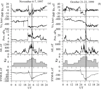
Fig. 1. Overview of the magnetic storms on (a) 6–7 November 1997 and (b) 21–23 October 1999. The solar wind and IMF data were obtained from Wind spacecraft taking into account the time shift of about 40 min. AE, Kp and SymH indices data were obtained from World Data Center C2 for Geomagnetism, Kyoto. Thick black vertical lines mark the time moment of minimum in SYM-H index through all panels at both figures.

influence the total proton ring current energy con-tent (evolution, peak values and location) during storm times?

2. How does the method of modeled SymH* calculation influence the magnitude and time history of this quan-tity during storms?

The paper is organized as follows. First, we present two storm events, one moderate (SymH minimum of−120 nT) on 6–7 November 1997, and one intense (SymH minimum of−230 nT) on 21–22 October 1999, which we have mod-eled. Section 3 presents our modeling approaches, includ-ing the description of the IMPTAM model and methods of model SymH* calculation used in this study. In Sects. 4 and 5 we present modeling results of the ring current energy pro-files, peak magnitudes and their UT locations for both storm events. In Sect. 6 we summarize our results and present the conclusions.

2 Overview of modeled storm events: 6–7 November 1997 and 21–23 October 1999

Two storm events were selected for the present study. Fig-ure 1 presents an overview of the magnetic storms on 6– 7 November 1997 and 21–23 October 1999. The solar wind and IMF data were obtained from the Wind spacecraft, in-cluding about 40 min time shift for propagation to the Earth’s magnetopause. The AE, Kp and SymH indices data were ob-tained from the World Data Center C2 for Geomagnetism, Kyoto.

[image:4.595.129.466.63.364.2]

(5)

The SymH index (sixth panel) reached −120 nT at about 04:00 UT on 7 November and recovered to−20 nT by the end of the day.

Figure 1b shows an overview of the intense storm on 21– 23 October 1999. IMFBz(first panel) turned from+20 nT to −20 nT at about 23:50 UT on 21 October and after some in-crease during the next three hours dropped to−30 nT around 06:00 UT on 22 October. After that, the IMF Bz oscil-lated around zero. TheVxcomponent of solar wind velocity (second panel) increased rather gradually from 480 km s−1 at 20:10 UT on 21 October up to 700 km s−1 at 02:58 UT on 22 October. Solar wind dynamic pressure (third panel) showed two main peaks, a 15 nPa peak around 24:00 UT on 21 October and a 35 nPa peak around 07:00 UT on 22 Octo-ber. There were several peaks in the AE index (fourth panel) reaching 800–1600 nT. The Kp index (fifth panel) increased to 5 from 03:00 to 06:00 UT on 21 October, and reached 8 during the storm maximum around 06:00 UT on 22 October. The SymH index (sixth panel) dropped to−230 nT at 06:00– 07:00 UT on 22 October. Thick black vertical lines mark the time moment of minimum in the SymH index in both figures.

3 Modeling approach

3.1 Inner magnetosphere particle transport and accel-eration model

The inner magnetosphere particle transport and acceleration model (IMPTAM), developed by Ganushkina et al. (2001, 2005, 2006), follows distributions of ions and electrons with arbitrary pitch angles from the plasma sheet to the inner L-shell regions with energies reaching up to hundreds of keVs in time-dependent magnetic and electric fields. We trace a distribution of particles in the guiding center, or drift, ap-proximation, in which we can picture the motion of a charged particle as displacements of its guiding center, or the center of the circular Larmor orbit of a moving particle. The guid-ing center theory assumes that the electromagnetic fields are known and can be used in geophysical plasmas, where the external field is strong and will not be changed much by the motion of the particle themselves.

As guiding center drifts we take into accountE×Bdrift, whereEandBare electric and magnetic fields, respectively, and magnetic drift, which, in its turn, includes gradient and curvature drifts. The drift velocity is a combination of the velocityVE×Bdue toE×BdriftVE×B=(E×B)/B2and the velocities of gradientV∇ and curvatureVcurdriftsV∇+ Vcur=(mv⊥2)/(2qB

2₎₍_B_{× ∇}_B)₊_(mv2 k)/(qR

2

cB2)(Rc×B) (Roederer, 1970), wheremis the particle mass,qis the par-ticle charge, v⊥ and vk are the particle velocities perpen-dicular and parallel to the magnetic field, respectively, Rc is the radius of curvature of magnetic field line (∇_⊥B= −(B/Rc)n, wherenis the unit normal vector along the ra-dius of curvature).

We assume that the first and second adiabatic invariants are conserved. The first adiabatic invariant for nonrela-tivistic particles is the particle magnetic moment given by µ=p2_⊥/(2mB), wherep⊥=p is the particle’s momentum in the guiding center system (Roederer, 1970). The magnetic moment of a particle is conserved in all cases, even in non-stationary fields, as long as the guiding center approximation is valid. There are two main conditions for guiding center approximation:

1. Spatial variations in the area of Larmor radius ρc are very small, so thatρc(∇⊥B/B)1. Magnetic fieldB does not vary much along the Larmor orbit.

2. Temporal variations are small in comparison with Lar-mor periodτc(∇⊥B/B)1.

Second adiabatic invariant is related to the bounce motion of a particle along magnetic field line. The integralJ=Hpkds, taken along a given fixed magnetic field line for a complete bounce cycle, wherepkis the particle’s momentum parallel to the magnetic field, anddsis the length element of a field line, is an adiabatic invariant and is conserved during the drift of a trapped particle as long as field variations during the time of a bounce periodτbare small(τbdB/dt )/B1. The particle’s momentum p is constant during one bounce, so J=2pI, whereI=RS

0 m

Sm[1−B(s)/Bm] 1/2_ds_,_S

mandS0mare the mirror points,B(s)is the magnetic field along magnetic field line,Bmis the magnetic field at the mirror point.

With the above mentioned assumptions, we consider bounce-average drift velocity after averaging over one bounce ofE×Bmagnetic drift velocities (Roederer, 1970)

hv0i =

E0×B0 B₀2

+ 2p

qτbB0

∇I×e0, (1)

whereE0andB0are the electric and magnetic fields in the equatorial plane, respectively,e0is the unit vector in the di-rection of the magnetic fieldB0.

In order to follow the evolution of the particle distribution functionf and particle fluxes in the inner magnetosphere de-pendent on the positionR, timet, energyEkin, and pitch an-gleα, it is necessary to specify:

1. particle distribution at initial time at the model boundary;

2. magnetic and electric fields everywhere dependent on time;

3. drift velocities;

4. all sources and losses of particles.

(6)

is the time,Ekinis the particle energy,αis the particle pitch angle, are obtained by solving the following equation:

df dt =

∂f ∂φ·Vφ+

∂f

∂R·VR+sources−losses, (2) whereVφ andVR are the azimuthal and radial components of the bounce-average drift velocity.

At the beginning of modeling with IMPTAM, the inner magnetosphere is considered empty. In this case, only the effects of newly entering particles from the plasma sheet are investigated. Ganushkina et al. (2006) have studied the ef-fects of the initial distribution on the storm-time ring current formation. For the 21–25 April 2001 storm, the modeling with an initially filled inner magnetosphere resulted in an in-crease by a factor of about 1.7 of the peak magnitude of the total proton ring current energy. The preexisting particles are subject to loss quickly after the newly injected particles oc-cupy the inner magnetosphere.

The model boundary is set in the plasma sheet at distances, depending on the scientific questions we are trying to answer, from 6.6REto 10RE. The particle distribution at the bound-ary is defined as a Maxwellian or kappa distribution func-tion with parameters obtained from the empirical relafunc-tions or from the observations during specific events.

Liouville’s theorem states that, in the absence of external forces and losses, the distribution function remains constant along the dynamic trajectory of particles. This theorem is used to gain information of the entire distribution function. If we know the distribution functionf (R,φ,t,Ekin,α)of par-ticles at a time momentt1, then we can obtain the distribu-tion funcdistribu-tion of particles at a time momentt2=t1+1t, by computing the drift velocity of the particles. The distribution function att2will not be the same as att1at the correspond-ing positions, since we need to take into account the phase-space-dependent losses (τloss). The final distribution function att2will bef (t2)=f (t1)exp(−1t /τloss).

Particle loss processes, which are important for modeling the ring current ions, include charge-exchange with neutral hydrogen in the upper atmosphere, Coulomb collisions, and convective outflow through the magnetopause. The charge-exchange cross-section is obtained from Janev and Smith (1993). The thermosphere model MSISE 90 (Hedin, 1991) and the plasmasphere model by Carpenter and Anderson (1992) are used.

An advantage of the IMPTAM is that it can simulate the full pitch-angle distribution of particles and utilize any mag-netic or electric field configurations (see below the list of rep-resentations used in the present study). In addition to the large-scale fields, transient fields associated with the dipolar-ization process in the magnetotail during substorm onset are included as an earthward propagating electromagnetic pulse of localized radial and longitudinal extent (Li et al., 1998; Sarris et al., 2002). The magnetic field disturbance from this dipolarization process was obtained from Faraday’s law. One of the important results obtained from IMPTAM modeling

is the ability to simulate several pulses launched at succes-sive substorm onset times (Ganushkina et al., 2001, 2005, 2006) to reproduce the observed amount of ring current pro-tons with energies>80 keV during a storm recovery phase (Ganushkina et al., 2006), which could not be achieved using other models for the magnetic field and large-scale convec-tion electric field.

IMPTAM has also been used (Ganushkina et al., 2004, 2005, 2006) to examine the evolution of the current systems during magnetic storms, to compute energetic ion drifts in the inner magnetosphere, and to evaluate the magnetospheric sources of magnetic disturbances recorded on ground (i.e., the sources of the Dst index).

3.2 Representations for magnetic and electric fields and boundary conditions used in simulations

The evolution of modeled proton distributions was followed using combinations of several representations for magnetic and electric fields with different boundary conditions. We use a dipole for the internal magnetic field. For the external magnetic field four different representations were used:

1. no external field sources (dipole only);

2. Kp-dependent Tsyganenko T89c (T89 abbreviation is used throughout the paper) (Tsyganenko, 1989; Peredo et al., 1993);

3. T96 (Tsyganenko, 1995) with Dst,Psw, IMFByandBz as input parameters;

4. Tsyganenko and Sitnov TS04 (Tsyganenko and Sitnov, 2005) with Dst,Psw, IMFByandBz and six variables Wi,i=1,6 as input parameters. The variablesW en-ter in the six magnitude coefficients for the magnetic fields from each source and calculated as time integrals dependent on solar wind and IMF parameters from the moment in time when IMFBzturns southward. The electric field representations include

1. Kp-dependent Volland-Stern VS (Volland, 1973; Stern, 1975) convection electric field;

2. Boyle et al. (1997) polar cap potential dependent on so-lar wind and IMF parameters applied to Volland-Stern type convection electric field field.

Four types of boundary proton distributions used in the model are the following:

1. BC1: Maxwellian distribution function at 6.6RE with n=0.5 cm−3andT=5 keV;

(7)

0 1 2 3 4 5

T

o

ta

l ri

ng c

u

rr

ent

ener

g

y

,

10

30

ke

V

November 6-7, 1997, IMPTAM model

0 1 2 3 4 5

dipole T89

T96 TS04

(a)

(b)

0 4 8 12 16 20

T

o

ta

l r

ing c

u

rr

ent

ener

gy

, 10

30

ke

V

0 4 8 12 16 20

(c)

(d) BC1: Maxwell at 6.6 Re, n=0.5 cm-3, T=5 keV BC2: kappa at 6.6 Re, n, T|| and T⊥ from LANL

0 10 20 30 40 50

0 6 12 18 0 6 12 18 24 Nov 6, 97 Nov 7, 97 UT

0 10 20 30 40 50

(f)

(e) (g)

0 10 20 30 40 50 0 10 20 30 40 50

(h) BC3: Maxwell at 10 Re, T= 5 keV, nps=0.025nsw+0.395 BC4: Maxwell at 10 Re, T, n from Tsyganenko and Mukai (2003)

B field E field

VS: Volland-Stern Boyle: Boyle et al. (1997)

Boundary conditions

BC1, VS

BC1, Boyle

BC2, VS

BC2, Boyle

BC3, VS BC4, VS

BC3, Boyle BC4, Boyle

-120 -80 -40 0 40

Sy

m

H

*,

n

T

-120 -80 -40 0 40

Sy

m

H

*,

n

T

0 6 12 18 0 6 12 18 24 Nov 6, 97 Nov 7, 97 UT

[image:7.595.125.471.65.578.2]

(i) (j)

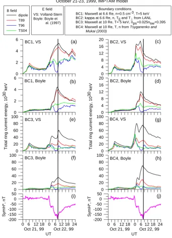
Fig. 2. Modeled proton (1–300 keV) ring current energy content during the 6–7 November 1997 storm with initially empty magnetosphere for combinations of four boundary conditions, two electric and four magnetic field representations. The corrected SymH* index is shown by thick purple lines. Thick black vertical lines mark the time moment of minimum in SymH* index through all figures. Note the scale differences on the panels.

part of the boundary (18:00–06:00 MLT) in the equato-rial plane;

3. BC3: Maxwellian distribution function at 10RE with parameterngiven by the empirical relation between the plasma sheet number density and the solar wind

num-ber densitynps=0.025nsw+0.395 (Ebihara and Ejiri, 2000) andT=5 keV;

(8)

0 2 4 6

T

o

tal ring current

energy, 10

30

keV

October 21-23, 1999, IMPTAM model

0 2 4 6 B field

dipole T89 T96 TS04

(a)

(b)

(c)

0 4 8 12 16 20

Tota

l ring current

en

erg

y

, 10

30

ke

V

0 4 8 12 16 20

(d)

0 20 40 60 80 100

0 6 12 18 0 6 12 18 24 Oct 21, 99 Oct 22, 99 UT

0 20 40 60 80 100

(e)

0 20 40 60 80 100 0 20 40 60 80 100

(g)

(h) (f)

-200 -150 -100 -50 0 50

Sy

m

H

*,

n

T

BC1: Maxwell at 6.6 Re, n=0.5 cm-3, T=5 keV BC2: kappa at 6.6 Re, n, T|| and T⊥ from LANL BC3: Maxwell at 10 Re, T= 5 keV, nps=0.025nsw+0.395 BC4: Maxwell at 10 Re, T, n from Tsyganenko and Mukai (2003)

E field VS: Volland-Stern Boyle: Boyle et al. (1997)

Boundary conditions

BC1, VS

BC1, Boyle

BC2, VS

BC2, Boyle

BC3, VS BC4, VS

-200 -150 -100 -50 0 50

Sy

m

H

*,

n

T

0 6 12 18 0 6 12 18 24 Oct 21, 99 Oct 22, 99 UT

[image:8.595.125.468.66.539.2]

(i) (j)

Fig. 3. Similar to Fig. 2 but for intense storm on 21–22 October 1999.

3.3 Methods of calculation of model Dst index

The corrected Dst* includes the pressure correction (Burton et al., 1975) and the contribution from induced currents Dst∗=Dst−7.26

√

Psw+11.0

1.3 (3)

with removed influence of the magnetopause currents (7.26√Psw), a correction factor for the contribution from in-duced currents within the Earth (1.3) (H¨akkinen et al., 2002) and a quiet-time offset value (11.0 nT) also taken into ac-count. We assume that the remaining contents of Dst* mainly

consist of the contributions from the ring and the tail cur-rents. We use the corrected 1 min SymH* index for our com-parisons, instead of the 1 h Dst* index, to have better time resolution.

Two different methods are used for our calculations of the modeled SymH* time series. One of them is the widely used Dessler-Parker-Sckopke relation DPS (Dessler and Parker, 1959; Sckopke, 1966)

(9)

0 1 2 3 4 5

R

C

E

m

ax

, 10

30

ke

V

E field

Volland-Stern Boyle et al. (1997)

dipole T89 T96 TS04

0 10 20 30 40 50

RCE

m

a

x, 1

0

30

ke

V

0 10 20 30 40 50

BC1

BC1: Maxwell at 6.6 Re, n=0.5 cm-3, T=5 keV BC2: kappa at 6.6 Re, n, T|| and T⊥ from LANL BC3: Maxwell at 10 Re, T= 5 keV, nps=0.025nsw+0.395 BC4: Maxwell at 10 Re, T, n from Tsyganenko and Mukai (2003)

Boundary conditions

BC2

BC3 BC4

(a) (b)

[image:9.595.128.463.66.318.2]

(c) (d)

Fig. 4. Peak magnitudes of the ring current energy profiles shown in Fig. 2 during 6–7 November 1997 storm.

which relates the total energy content ERC of the plasma within the inner magnetosphere to a magnetic perturbation at the center of the Earth SymH∗_DPS.

Another method uses the Biot-Savart law to derive the magnetic disturbance induced by the current. The current densityJ⊥perpendicular to the magnetic fieldBis given by

J⊥= B

B2×

∇P⊥+(Pk−P⊥)

(B· ∇)B

B2

, (5)

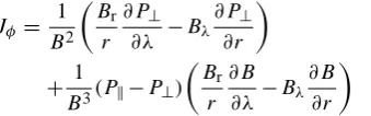
wherePkandP⊥are plasma pressure, parallel and perpen-dicular to the magnetic field. This equation is valid if a quasi-static equilibrium exists (force balanced state) and there is no time dependence on the timescale of interest and inertial terms can be neglected. The magnetic disturbance parallel to the Earth’s dipole at the center of the Earth4Bis induced by the azimuthal componentJφofJ⊥

4B=µ0

4π

Z

r

Z

λ

Z

φ

cos2λJφ(r,λ,φ)drdλdφ, (6)

whereµ0 is the magnetic permeability, r is the radial dis-tance,λis the latitude,φis the MLT andJφis given by

Jφ = 1 B2

_B

r r

∂P⊥ ∂λ −Bλ

∂P⊥ ∂r

+ 1

B3(Pk−P⊥)

_B

r r

∂B ∂λ−Bλ

∂B ∂r

(7)

and4Bis an estimate of the corrected SymH* index.

4 Modeling results: ring current energy content

4.1 Ring current energy profiles

Figure 2 shows the evolution of modeled proton ring current energy in units of 1030_{keV during the 6–7 November 1997} storm for several combinations of the magnetic and elec-tric fields and boundary conditions. At each panel (a–h) the ring current energy computed using different magnetic fields is shown by different colors: dipole (thick black lines), T89 (red lines), T96 (blue lines), and TS04 (green lines). The corrected SymH* index (i, j) with pressure correction and with quiet-time offset and removed contribution from induced currents within the Earth is shown by thick purple lines. Thick black vertical lines mark the time of minimum SymH* through all figures. Note that the scales are different for panels (a), (b), (c), (d) and (e)–(h), but they are the same for the same boundary conditions but different electric fields (a and b for BC1), (c and d for BC2) and for all combinations for BC3 and BC4.

Figure 3 shows, similarly to Fig. 2, the evolution of mod-eled proton ring current energy in 1030keV during the 21– 22 October 1999 intense storm for several combinations of magnetic and electric fields and boundary conditions.

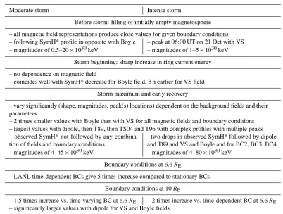
[image:9.595.49.219.644.697.2]

(10)

[image:10.595.94.497.82.386.2]

Table 1. Model-dependent storm-time ring current: ring current energy profiles.

Moderate storm Intense storm

Before storm: filling of initially empty magnetosphere

– all magnetic field representations produce close values for given boundary conditions – following SymH* profile in opposite with Boyle – peak at 06:00 UT on 21 Oct with VS – magnitudes of 0.5–20×1030keV – magnitudes of 1–5×1030keV

Storm beginning: sharp increase in ring current energy

– no dependence on magnetic field

– coincides well with SymH* decrease for Boyle field, 3 h earlier for VS field

Storm maximum and early recovery

– vary significantly (shape, magnitudes, peak(s) locations) dependent on the background fields and their parameters

– 2 times smaller values with Boyle than with VS for all magnetic fields and boundary conditions – largest values with dipole, then T89, then TS04 and T96 with complex profiles with multiple peaks – observed SymH* not followed by any

combina-tion of fields and boundary condicombina-tions

- two drops in observed SymH* followed by dipole and T89 and VS and Boyle and for BC2, BC3, BC4 – magnitudes of 4–45×1030keV – magnitudes of 4–80×1030keV

Boundary conditions at 6.6RE

– LANL time-dependent BCs give 5 times increase compared to stationary BCs

Boundary conditions at 10RE

– 1.5 times increase vs. time-varying BC at 6.6RE – 2 times increase vs. time-dependent BC at 6.6RE – significantly larger values with dipole for VS and Boyle fields

4.2 Peak magnitudes of the ring current energy and their UTs

In order to better examine and highlight the similarities and differences between the model configurations within IMP-TAM, the results were distilled to only the peak magnitudes of the ring current intensity. Figure 4 presents these peak magnitudes in units of 1030keV of the ring current energy profiles shown in Fig. 2 during the 6–7 November 1997 storm for four boundary conditions (BC1-BC4) for the Volland-Stern (open diamonds) and the Boyle (black diamonds) elec-tric fields as dependent on four magnetic fields (dipole, T89, T96, and TS04). Peak magnitudes of the ring current en-ergy profiles for the intense 21–22 October 1999 storm are shown in Fig. 5 similarly to those for the moderate storm on 6–7 November 1997 (Fig. 4).

Another distillation of the time series plots in Figs. 2 and 3 is to consider the offset in Universal Time (UT) between the peak of the modeled ring current energy content and the SymH* minimum. Figure 6 presents the times of the peak magnitudes of the ring current energy profiles shown in Fig. 2 during the 6–7 November 1997 storm in terms of the difference1UTRCE=UT(RCEmax)−UT(SymHmin)between UT(RCEmax), when the maximum of the ring current en-ergy is reached during the storm and UT(SymHmin), when

the SymH* index dropped to its minimum. Negative values of1UTRCEmean before and positives values mean after the storm maximum as defined by the UT of the SymH* mini-mum, respectively. It is worth mentioning that the locations of peak values of the ring current energy can be determined rather easily for the dipole and T89 magnetic field, whereas it is more difficult to do when using the T96 and TS04. The ring current energy profiles for the T96 and TS04 exhibit more variations and peaks. In the present study in Figs. 4 and 6 the largest peaks are plotted.

Locations of the peak magnitudes of the ring current en-ergy profiles during the intense 21–22 October 1999 storm are presented in Fig. 7 similarly to Fig. 6.

Table 2 contains the main features of the storm-time ring current energy peak values and their UTs for both storm events, moderate on 6–7 November 1997 and intense on 21– 22 October 1999.

5 Modeling results: global magnetic field depression

5.1 Model SymH* profiles computed by Biot-Savart and Dessler-Parker-Sckopker DPS relation methods

(11)

0 2 4 6 8 10

RCE

m

a

x

, 1

0

30

ke

V

E field

0 20 40 60 80

RCE

m

a

x

, 1

0

30

ke

V

0 20 40 60 80

BC1

BC1: Maxwell at 6.6 Re, n=0.5 cm-3, T=5 keV BC2: kappa at 6.6 Re, n, T|| and T⊥ from LANL BC3: Maxwell at 10 Re, T= 5 keV, nps=0.025nsw+0.395

BC4: Maxwell at 10 Re, T, n from Tsyganenko and Mukai (2003)

Boundary conditions

BC2

BC3 BC4

(a) (b)

[image:11.595.129.469.69.327.2]

(c) (d)

Fig. 5. Peak magnitudes of the ring current energy profiles shown in Fig. 3 during 21–22 October 1999 storm, similar to Fig. 4.

-6 -4 -2 0 2 4 6

UT

(RCEmax) - UT(SymHmin), hour

E field

-6 -4 -2 0 2 4 6

UT

(R

CEmax) - UT(SymHmin), hour

-6 -4 -2 0 2 4 6

BC1

Boundary conditions

BC2

BC3 BC4

(a) (b)

[image:11.595.128.468.369.617.2]

(c) (d)

Fig. 6. Times of the peak magnitudes of the ring current energy profiles shown in Fig. 2 during 6–7 November 1997 storm in terms of the difference1UTRCE=UT(RCEmax)−UT(SymHmin)(see the text).

magnetic perturbation for direct comparison with SymH*. Figure 8 presents the modeled SymH* computed as mag-netic field depression at the center of the Earth produced by

(12)

-8 -6 -4 -2 0 2

UT

(RCEmax) - UT(SymHmin), hour

E field

-8 -6 -4 -2 0 2

UT

(R

CEmax) - UT(SymHmin), hour

-8 -6 -4 -2 0 2

BC1

Boundary conditions

BC2

BC3 _BC4

(a) (b)

[image:12.595.127.461.67.315.2]

(c) (d)

Fig. 7. Times of the peak magnitudes of the ring current energy profiles shown in Fig. 3 during 21–22 October 1999 storm, similar to Fig. 6.

Table 2. Model-dependent storm-time ring current: peak values and their UTs.

Peak magnitudes

– peak magnitudes are, in general, quite similar for both moderate and intense storms – Boyle results in 2 times smaller peak values compared to VS for all magnetic fields and BCs – peak magnitudes decrease when moving from dipole to more realistic magnetic fields – 5 times increase from stationary to LANL

time-dependent BC at 6.6RE, further 2 times increase when moving from 6.6 to 10RE

– 5 times increase from stationary to LANL time-dependent BC at 6.6RE, further 3 times increase when moving from 6.6 to 10RE

– at 10REnot much difference for T89, T96 and TS04 for VS and Boyle fields UT differences of peak magnitudes and SymH* minima

– best coincidence for Boyle and dipole and T89, all BC, except for BC4 from Geotail at 10RE

–1UT_RCEclose to 0 for dipole and T89 and Boyle and for BC1, BC3 and BC4

– for BC1 and BC3, VS results in close to zero val-ues

– plus 2.5 h for all magnetic fields for VS for LANL time-dependent BC at 6.6 and 10RE (BC2, BC3 and BC4)

– Boyle gives1UTRCEvalues closer to zero than VS

– at 6.6REfor T96 and TS04, UT difference is+2 h for Boyle, at 10REis−2 h

– for T96 and TS04 and for VS, UT difference is −6 h for BC1-BC3

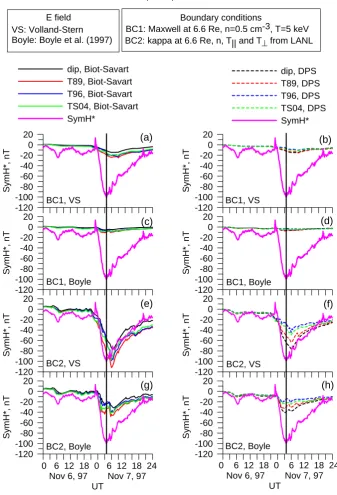
VS and Boyle electric fields were used. Panels on the right (Fig. 8b, d, f, h) were calculated using the Dessler-Parker-Sckopke DPS relation between the total ring current energy and the magnetic field depression produced by it at the cen-ter of the Earth. At each panel, the modeled SymH* was computed using several magnetic field representations such

(13)

-120 -100 -80 -60 -40 -20 0 20

SymH*, nT

dip, Biot-Savart T89, Biot-Savart T96, Biot-Savart TS04, Biot-Savart SymH*

-120 -100 -80 -60 -40 -20 0 20

Sy

m

H

*,

n

T

dip, DPS T89, DPS T96, DPS TS04, DPS SymH* November 6-7, 1997, IMPTAM model

0 6 12 18 0 6 12 18 24 Nov 6, 97 Nov 7, 97 UT

-120 -100 -80 -60 -40 -20 0 20

SymH*, nT

-120 -100 -80 -60 -40 -20 0 20

Sy

m

H

*,

n

T

0 6 12 18 0 6 12 18 24 Nov 6, 97 Nov 7, 97 UT

(a) _(b)

(c) (d)

-120 -100 -80 -60 -40 -20 0 20

Sym

H

*, nT

-120 -100 -80 -60 -40 -20 0 20

SymH*, nT

-120 -100 -80 -60 -40 -20 0 20

Sym

H

*, nT

-120 -100 -80 -60 -40 -20 0 20

Sym

H

*, nT

(e) (f)

(g) (h)

BC1: Maxwell at 6.6 Re, n=0.5 cm-3, T=5 keV

BC2: kappa at 6.6 Re, n, T|| and T⊥ from LANL

Boundary conditions E field

VS: Volland-Stern Boyle: Boyle et al. (1997)

BC1, VS BC1, VS

[image:13.595.127.465.71.567.2]

BC2, VS BC2, VS

Fig. 8. Magnetic field depression at the center of the Earth produced by the modeled proton (1–300 keV) distribution during 6–7 Novem-ber 1997 storm with boundary distribution at 6.6RE. Calculations were made by using Biot-Savart’s law and Dessler-Parker-Sckopke relation. The observed corrected SymH* index is shown by thick purple lines. Thick black vertical lines mark the time moment of minimum in the observed SymH* index through all panels.

used such as dipole (dashed black lines), T89 (dashed red lines), T96 (dashed blue lines), and TS04 (dashed green lines). The observed corrected SymH* index with quiet-time offset and removed contribution from induced currents within the Earth is shown by thick purple lines. Thick black vertical lines mark the time moment of the minimum in the

observed corrected SymH* through all panels. Figure 9 presents the modeled SymH*, similarly as Fig. 8 but for boundary conditions BC3 and BC4.

(14)

-200 -160 -120 -80 -40 0

SymH*, nT

-200 -160 -120 -80 -40 0

Sy

m

H

*,

n

T

dip, DPS T89, DPS T96, DPS TS04, DPS SymH* November 6-7, 1997 storm, IMPTAM model

0 6 12 18 0 6 12 18 24 Nov 6, 97 Nov 7, 97 UT

-200 -160 -120 -80 -40 0

SymH*, nT

-200 -160 -120 -80 -40 0

SymH*, nT

BC3, VS

0 6 12 18 0 6 12 18 24 Nov 6, 97 Nov 7, 97 UT

(a) (b)

(c) (d)

(f) -200

-160 -120 -80 -40 0

Sym

H

*, nT

-200 -160 -120 -80 -40 0

SymH*, nT

-200 -160 -120 -80 -40 0

Sym

H

*, nT

-200 -160 -120 -80 -40 0

Sym

H

*, nT

BC4, VS

BC4, VS (e)

(g) (h)

VS: Volland-Stern

Boyle: Boyle et al. (1997) BC3: Maxwell at 10 Re, T= 5 keV, nps=0.025nsw+0.395 BC4: Maxwell at 10 Re, T, n from Tsyganenko and

[image:14.595.130.470.68.563.2]

Mukai (2003)

Fig. 9. Similar to Fig. 8 but for boundary distribution at 10RE.

modeled proton (1–300 keV) distribution during the intense 21–22 October 1999 storm for boundary conditions BC1 and BC2, and BC3 and BC4.

Table 3 describes the results on the modeled SymH* com-puted using the Dessler-Parker-Sckopke DPS relation and Biot-Savart integration for both storm events, moderate on 6–7 November 1997 and intense on 21–22 October 1999.

5.2 Minima values and their UTs of model SymH* profiles

(15)

-200 -150 -100 -50 0 50

Sym

H

*, nT

-200 -150 -100 -50 0 50

SymH*, nT

dip, DPS T89, DPS T96, DPS TS04, DPS SymH* October 21-22, 1999 storm, IMPTAM model

-200 -150 -100 -50 0 50

Sym

H

*, nT

-200 -150 -100 -50 0 50

SymH*, nT

BC1, VS

(a) (b)

(c) (d)

-200 -150 -100 -50 0 50

SymH

*, nT

-200 -150 -100 -50 0 50

Sym

H

*, nT

0 6 12 18 0 6 12 18 24 Oct 21, 99 Oct 22, 99 UT

-200 -150 -100 -50 0 50

Sy

m

H

*,

n

T

-200 -150 -100 -50 0 50

SymH

*, nT

BC2, VS

0 6 12 18 0 6 12 18 24 Oct 21, 99 Oct 22, 99 UT

(e) (f)

(g) (h)

BC1: Maxwell at 6.6 Re, n=0.5 cm-3, T=5 keV

BC2: kappa at 6.6 Re, n, T|| and T⊥ from LANL

[image:15.595.128.465.68.550.2]

Fig. 10. Similar to Fig. 8 but for 21–22 October 1999 storm.

Volland-Stern (open diamonds) and Boyle (black diamonds) electric fields as dependent on the four magnetic field rep-resentations (dipole, T89, T96, and TS04). Figures in the left column were obtained by using the Biot-Savart law and figures in the right column by using the DPS relation for SymH* calculations. Purple horizontal lines mark the ob-served SymH* minimum value of−100 nT.

Figure 13 presents, similarly to Fig. 12, the minimum SymH* values of the modeled SymH* profiles shown in Figs. 10 and 11 during 21–22 October 1999 storm. Purple

horizontal lines mark the observed SymH* minimum value of−200 nT.

(16)

-300 -200 -100 0

SymH

*, nT

-300 -200 -100 0

Sym

H

*, nT

dip, DPS T89, DPS T96, DPS TS04, DPS SymH* October 21-22, 1999 storm, IMPTAM model

-300 -200 -100 0

SymH

*, nT

-300 -200 -100 0

Sym

H

*, nT

BC3, VS

(a) (b)

(c) (d)

-300 -200 -100 0

Sy

m

H

*,

n

T

-300 -200 -100 0

SymH

*, nT

0 6 12 18 0 6 12 18 24 Oct 21, 99 Oct 22, 99 UT

-300 -200 -100 0

SymH*, nT

-300 -200 -100 0

Sy

m

H

*,

n

T

BC4, VS

0 6 12 18 0 6 12 18 24 Oct 21, 99 Oct 22, 99 UT

(e) (f)

(g) (h)

VS: Volland-Stern

[image:16.595.136.469.72.535.2]

Boyle: Boyle et al. (1997) BC3: Maxwell at 10 Re, T= 5 keV, nps=0.025nsw+0.395 BC4: Maxwell at 10 Re, T, n from Tsyganenko and Mukai (2003)

Fig. 11. Similar to Fig. 9 but for 21–22 October 1999 storm.

before and positives values mean after the storm maximum as defined by the UT of SymH* minimum, respectively.

Figure 15 presents the UTs of the minimum SymH* values of the modeled SymH* profiles shown in Figs. 10 and 11 during 21–22 October 1999 storm, similar to Fig. 14.

Table 4 highlights the results of the minimum values and their UTs of modeled SymH* computed using the Dessler-Parker-Sckopker DPS relation and Biot-Savart integration for both storm events, moderate on 6–7 November 1997 and in-tense on 21–22 October 1999.

6 Discussion and conclusions

(17)

-30 -20 -10 0

SymH_min, nT

November 6-7, 1997 storm, IMPTAM model

-30 -20 -10 0

SymH_min, nT

-200 -160 -120 -80 -40 0

Sy

m

H

_m

in

, nT

BC4

-200 -160 -120 -80 -40 0

SymH_min, nT

-200 -160 -120 -80 -40 0

E field

Boundary conditions

BC4

BC3 BC3

BC2 BC2

BC1 BC1

SymH from Biot-Savart SymH from DPS

(a) (b)

(c) (d)

(e) (f)

[image:17.595.130.462.67.500.2]

(g) (h)

Fig. 12. Minimum SymH* values of the modeled SymH* profiles shown in Figs. 8 and 9 during 6–7 November 1997 storm. Purple horizontal lines mark the observed SymH* minimum value.

minimum of −230 nT) on 21–22 October 1999. In addi-tion, SymH* was computed from the results by two methods, the Dessler-Parker-Sckopke relation (DPS) and Biot-Savart’s law. We used varying but prescribed electric and magnetic fields, in which protons move, not taking into account self-consistency. It was done especially to investigate how much the modeled ring current depends on the background mag-netic and electric fields and boundary conditions used in sim-ulations and, correspondingly, how much can physical con-clusions made from simulations be dependent on them.

In our modeling the magnetosphere was empty at the be-ginning. The filling of the inner magnetosphere with parti-cles coming from the plasma sheet is seen for all combina-tions of magnetic and electric fields and boundary condicombina-tions.

(18)

-40 -30 -20 -10 0

SymH_min, nT

October 21-22, 1999 storm, IMPTAM model

-40 -30 -20 -10 0

SymH_min, nT

-300 -200 -100 0

Sy

m

H

_m

in

, nT

BC4

-300 -200 -100 0

SymH_min, nT

-300 -200 -100 0

E field

Boundary conditions

BC4

BC3 BC3

BC2 BC2

BC1 BC1

(a) (b)

(c) (d)

(e) (f)

(g) (h)

Fig. 13. Minimum SymH* values of the modeled SymH* profiles shown in Figs. 10 and 11 during 21–22 October 1999 storm. Purple horizontal lines mark the observed SymH* minimum value.

moderate storm, the magnitude of the ring current energy ac-cumulated during the modeling period before the storm does not depend much on the location of the model boundary (at 6.6 or at 10RE). It is roughly true for the intense storm too, except for the Kp-dependent peak.

The time when the ring current energy starts to increase sharply at the storm beginning does not depend on mag-netic field used and coincides quite well with the observed SymH* decrease for the Boyle field but occurs 3 h earlier for the VS field. Further evolution of the ring current energy profiles (in shape, magnitudes, peak(s) locations) strongly depend on the background fields and boundary conditions used. Less realistic magnetic field configurations (dipole and T89) give larger values than more realistic ones (T96

[image:18.595.128.462.65.501.2]

(19)

-6 -4 -2 0 2 4 6

November 6-7, 1997 storm, IMPTAM model

-6 -4 -2 0 2 4 6

UT(SymH_min

)

UT(S

ymH_

m

in_ob

s), h

our

BC4

-6 -4 -2 0 2 4 6

U

T

(SymH

_

min) - UT(SymH_m

in_ob

s), hour

-6 -4 -2 0 2 4 6

E field

Boundary conditions

BC4

BC3 BC3

BC2 BC2

BC1 BC1

(a) (b)

(c) (d)

(e) (f)

[image:19.595.130.458.70.496.2]

(g) _(h)

Fig. 14. UTs of the minimum SymH* values of the modeled SymH* profiles shown in Figs. 8 and 9 during 6–7 November 1997 storm in terms of the difference1UTSymH(see the text).

lead to an enhanced ring current (Chen et al., 2007; Lavraud and Jordanova, 2007).

With moving the model boundary to 10RE, additional in-crease by a factor of 1.5 for the moderate storm and a factor of about 2 for the intense storm is detected. This is consistent with previous results by Zheng et al. (2010) that a source that is farther away from the Earth leads to a stronger ring current. Setting the model boundary outside of 6.6REgives a possi-bility to take into account the particles in the transition region (between dipole and stretched field lines) forming the partial ring current and near-Earth tail current in that region. The dipole field produced significantly larger ring current energy compared to other magnetic fields. Assuming the magnetic

field to be a dipole inside 10RE provides easier access of plasma sheet particles to the ring current region.

(20)

-8 -6 -4 -2 0 2

October 21-22, 1999 storm, IMPTAM model

-8 -6 -4 -2 0 2

UT(SymH_min

)

UT(S

ymH_

m

in_ob

s), h

our

BC4

-8 -6 -4 -2 0 2

U

T

(SymH

_

min) - UT(SymH_m

in_ob

s), hour

-8 -6 -4 -2 0 2

E field

Boundary conditions

BC4

BC3 BC3

BC2 BC2

BC1 BC1

(a) (b)

(c) (d)

(e) (f)

[image:20.595.133.460.67.500.2]

(g) _(h)

Fig. 15. UTs of the minimum SymH* values of the modeled SymH* profiles during 21–22 October 1999 storm, similar to Fig. 14.

to the ring current energy profiles (Figs. 2 and 3). When the Biot-Savart method is used, the order is different: the largest absolute SymH* values are with the T89 field, and absolute SymH* magnitudes calculated with a dipole can be close to those of T96 and TS04 with some variations. This reflects the fact that when using Biot-Savart’s law, the modeled SymH* is not assumed to come from the ring current energy only.

Figure 16 shows the differences 1SymH* between SymH* calculated by Biot-Savart’s law and DPS relation for both storms, for all model combinations and for LANL time-dependent BC2 at 6.6REand BC4 at 10RE. It can be seen that for dipole magnetic field the difference are mainly posi-tive before the storm and for the beginning storm main phase for both VS and Boyle electric fields and BC2 and BC4. It

means that DPS gives smaller SymH* values (larger in ab-solute values) than Biot-Savart’s law. Here we need to re-member how DPS is calculated and with what assumptions following Liemohn (2003) study.

DPS relation was derived for the dipole field (1B_B

E

=

−2ERC

3UE , whereBE is the equatorial surface magnetic field

(21)

-60 -40 -20 0 20

-Sy

m

H

*,

n

T

dip, SymH*(Biot-Savart) -SymH*(DPS) T89, SymH*(Biot-Savart) - SymH*(DPS) T96, SymH*(Biot-Savart) - SymH*(DPS) TS04, SymH*(Biot-Savart) - SymH*(DPS)

0 6 12 18 0 6 12 18 24 Nov 6, 97 Nov 7, 97

(e) (g)

(f) (h)

-60 -40 -20 0 20

-SymH*, nT

-100 -80 -60 -40 -20 0 20 40

-SymH*, nT

-60 -40 -20 0 20

-SymH*,

nT

-100 -80 -60 -40 -20 0 20 40

-SymH*

, nT

(a) (c)

(b) (d)

BC2: kappa at 6.6 Re, n, T|| and T⊥ from LANL Boundary conditions E field

BC2, VS BC4, VS

BC4: Maxwell at 10 Re, T, n (Tsyganenko and Mukai, 2003)

0 6 12 18 0 6 12 18 24 Oct 21, 99 Oct 22, 99

0 6 12 18 0 6 12 18 24 Oct 21, 99 Oct 22, 99 -60

-40 -20 0 20 40

-SymH*

, nT

-120 -80 -40 0 40 80

-SymH*, nT

-120 -80 -40 0 40 80

-SymH*,

[image:21.595.127.464.61.528.2]

nT

Fig. 16. Differences between model SymH* calculated by Biot-Savart’s law and DPS relation for moderate 6–7 November 1997 and intense 21–22 October 1999 storm events.

truncation current implicitly included in the DPS relation is, in some qualitative sense, accounting for the tail current or any current beyond the outer boundary.” When we calculate SymH* by Biot-Savart’s law for dipole magnetic field, we do not include this current, so SymH* calculated by Biot-Savart’s law is larger (smaller in absolute values) than that by DPS.

When we calculate SymH* by Biot-Savart’s law in Tsyga-nenko magnetic fields, we include the effect from the near-Earth tail current by including the effect from the stretched magnetic field lines for both boundaries at 6.6 and 10RE.

DPS relation also contains some sort of contribution from other currents than the ring current but incorrectly. Espe-cially, when the ring current energy used in the DPS relation is calculated following particles in the nondipolar magnetic field, but other magnitudes are still obtained from the dipole field.

(22)

[image:22.595.96.508.115.481.2]

Table 3. Model-dependent storm-time ring current: modeled SymH* index.

Biot-Savart DPS Biot-Savart DPS

Boundary conditions at 6.6RE

– for all fields (except dipole) and BCs modeled|SymH*|by DPS are smaller than those by Biot-Savart law – for stat. BC all fields give 10 times smaller than observed at min|SymH*|by DPS and Biot-Savart

– modeled SymH* for all fields does not follow ob-served SymH*

– for VS and dipole, T96 and TS04 follow closely first dip in SymH* and plateau

– dipole and T89 gave closest to observed first SymH* dip

– largest |SymH*| by T89, then TS04, T96, dipole

– largest |SymH*| by dipole, then T89, TS04, T96

– largest |SymH*| by T89, then dipole, TS04, T96

largest |SymH*| by dipole, then T89, TS04, T96

– two minima before the storm not reproduced – no combination of fields and BCs able to follow observed SymH* and reproduce min SymH* – best in min values and

recovery: VS, T96 and TS04 for BC2

– smaller than observed with late min for BC2

– Boyle field results in 2 times smaller than the observed of min|SymH*|

Boundary conditions at 10RE – for VS and dipole and

T89 |SymH*| 2 times larger

– for VS and all magnetic fields 2 times smaller of |SymH*|

– exception: dipole: 60 nT min |SymH*| overestimate

– except for BC3 and Boyle, dipole largerly overes-timates|SymH*|

– for all magnetic fields and VS, SymH* drops 2 h earlier than observed – for Boyle and all

magnetic fields SymH* follow observed before storm and SymH drop, not storm max

– only−40 nT by dipole, compared to−100 nT

– for BC3 and Boyle and dipole, model SymH* follow most closely observed

– T96 and TS04 the worst for all combinations of fields to follow the observed SymH*

condition for moderate 6–7 November 1997 storm (Fig. 16a– d). For intense storm on 21–22 October 1999 (Fig. 16e–h), the situation is generally the same, except for the variations when using T96 model discussed previously in the present paper.

Different combinations of fields and boundary conditions result in different modeled SymH*. For the moderate storm and using Biot-Savart’s law, the closest modeled SymH* profiles to the observed one were obtained for LANL time-dependent boundary conditions at 6.6REfor VS electric field and T96 and TS04 magnetic fields (Fig. 8e). In Fig. 8, none of the modeled SymH* profiles follow the sharp decrease (they are not sharp enough) in the observed SymH* and they eventually reach minimum 2–3 h after the observed mini-mum. With Biot-Savart’s law inside 10RE, the modeled ab-solute SymH* values are overestimated for the VS field and all magnetic fields. The VS field is not suitable here, and also

the boundary conditions at 10REare far from being realistic, even though the plasma sheet moments depend on IMF and solar wind parameters.

(23)

[image:23.595.91.510.86.402.2]

Table 4. Model-dependent storm-time ring current: minimum values and their UTs of model SymH*.

Biot-Savart DPS Biot-Savart DPS

Minimum values of model SymH*

– VS produced larger values of min|SymH*|than Boyle for all magnetic fields and BCs – for stationary BC min |SymH*| are in−25 to

−5 nT

– for BC at 6.6REmin|SymH*|smaller than ob-served, 10 times BC1 and 2 times for BC2 – closest to observed

min|SymH*|for BC2 at 6.6RE and VS and T96 and TS04

– no close to observed min SymH*, best for VS and T89 with BC at 10RE

– close to observed for VS, T96 and TS04, and dipole and Boyle for BC4

– closest to observed for VS and T96 and TS04 for BC4

– not much dependence on magnetic field for min |SymH*|with Boyle field

– significant min |SymH*| overestimates for VS and all magnetic fields for BC at 10RE

– significant min |SymH*| overestimates for VS and dipole for BC at 10RE

– with BC at 10REdipole resulted in min|SymH*| 50–100 nT larger than observed for VS

UT differences of model minimum SymH*

– for VS min SymH* 2–5 h after observed for all magnetic fields and BCs

– for stationary BC similar for VS and Boyle and all magnetic fields

– smallest1UT_SymHfor Boyle and dipole and T89 for BC1 and BC3

– smallest1UT_SymHfor Boyle and dipole and T89 for BC1, BC2 and BC3

– close to zero1UT_SymHfor Boyle and dipole and T89 for BC1, BC3 and BC4

– at 10RE1UTSymHrather similar for given BC – at 10REfor T96 and TS04 modeled storm max occurred 2 h for Boyle field

– at 10REfor T96 and TS04 modeled storm max occurred much earlier (6 to 8 h) for VS and Boyle

SymH* values due to the easier access of plasma sheet parti-cles to the ring current region.

For the intense storm, no combination was able to repro-duce the two-step decrease in the observed SymH*, only one combination (of Boyle, T89 and BC4 boundary condi-tions at 10RE) resulted in relatively close magnitudes. Note that using the T96 and TS04 magnetic fields resulted in very unrealistic SymH* profiles with peaks even at the observed SymH* minimum. The magnetic field configuration in the inner magnetosphere during the intense storm on 21–22 Oc-tober 1999 was modeled by using different magnetic fields by Kalegaev et al. (2005). It was shown that the Tsyganenko T02 field (Tsyganenko, 2002) underestimated theBz compo-nent significantly (by 100 nT) at the storm maximum com-pared to GOES 8 and GOES 10 measurements. GOES 8 was around midnight and GOES 10 was moving toward midnight in the dusk sector. This indicates that precautions must be taken when using realistic yet empirical magnetic fields in real storm event modeling. It is always good to compare the observed magnetic field with the modeled one for an event to be modeled, when globally applying a magnetic field config-uration to the magnetosphere.

In general, the structure of the observed SymH* profiles during the intense storm is better reproduced than during the moderate storm, even using the DPS method, although the actual magnitudes are not the same. It follows the previous modeling results by Ganushkina et al. (2004) that during in-tense storms, the tail current is intensified, but the main con-tribution comes from the ring current. Note that Ganushk-ina et al. (2004) modeling was conducted using the event-oriented magnetospheric magnetic field representation tech-nique based on actual magnetic field measurements for sev-eral events, and in the present paper we employ the particle model IMPTAM.

Keeping the points discussed above in mind the conclu-sions are as follows:

1. Different combinations of the magnetic and electric fields and boundary conditions result in very different modeled ring current, and, therefore, the physical con-clusions based on simulation results can differ signifi-cantly.