An Analytic Approach to Scheduling Pipe Replacement

Full text

(1)An Analytic Approach to Scheduling. Pipe Replacement Uri Shamir and Charles D.D. Howard. 248. MANAGEMENT AND OPERATIONS. A procedure is described that uses the history of main breaks to forecast how the number of breaks would change with time if the pipe were not replaced; a separate analysis predicts the failure rate of newly installed pipes. These forecasts are combined with cost data and a discount rate that accounts for inflation to determine the optimal replacement date.. Water main breaks are a problem of concern to many water supply agencies. Breaks cause disruption in service, pose a potential danger when they reduce temporarily fire fighting capabilities, may cause damage to other services and to property, and incur substantial repair costs. Breaks may also cause a disruption in the normal work schedule and create an atmosphere of public concern that pressures the water supply agency. When a pipe breaks, the leak has to be located, the pipe exposed, and the leak fixed or a section replaced. When a length of pipe shows an increasing susceptibility to breaks, consideration should be given to replacing it entirely with a new pipe. The reasons for breaks are many and can be classi fied in several categories: 1. The quality and age of the pipe itself, including connectors and other equipment 2. The type of environment in which the pipe is laid e.g., the corrosivity of the soil, frost and heaving, external loads 3. The quality of the workmanship used,in laying the pipe 4. The service conditions, such as pressure and water hammer. An analysis of break data may help pinpoint the main reasons for breaks in a certain area of the network or in a specific pipe. Changes in pipeline design and construction policies may then be issued. This, how ever, does not solve the problem of a pipeline that is in service and exhibits a history of many breaks. There are essentially two ways of dealing with such a situa tion: to either repair or to replace the pipe. A rational decision to replace or not to replace a pipe at a particular time must be based on a comparison of the two alternatives: whether to replace the pipe, incurring the replacement cost and whatever future costs are associated with the new line, or to retain the existing length of pipe, at least for the time being, saving the replacement cost but incurring possible future costs of repair, disruption of service, and damages. The analysis required for such a decision must include a projection. 0003-150X/79/050248-11 $01.00 ©1979 American Water Works Association. JOURNAL AWWA.

(2) of the expected rate of breaks in the two pipes the existing one and the potential replacement. This paper presents a method for determining the optimal time to replace a pipe. To carry out the analysis, break data must be examined and used to forecast how the number of breaks in the existing pipe is going to change over time. Next, it is necessary to estimate the number of breaks that would occur in a replacement length of pipe. By combining these fore casts with economic data for replacing the pipe and for fixing a break, the optimal replacement date can be determined. Water utilities should record for each break all the information needed to carry out an evaluation of breaks and their causes. Some attempts have been made to correlate break data with possible causes, such as soil type, soil temperatures at the pipe depth, service pressures, water hammer, and external loads. Different zones of the distribution system may have to be analyzed separately to account for local conditions. The information gained from such a cause-effect study aids in making long-term policy decisions regarding selection of pipe materials, coating, cathodic protec tion, and construction procedures. It may also influence the immediate operational decision on pipe replacements. To develop a general method for deter mining optimal replacement policies it is not necessary to determine the cause of breaks, only how they are expected to progress in the future. One of the key components in the method to be used is a realistic estimate of future rates of failure, and for this purpose a cause-effect study may be very important. Analysis of Break Data. Breaks in the existing pipe. A convenient way to measure the number of breaks is in breaks per year per 1000 ft of pipe. Other time periods can be used, if there are data to show, for example, differences between summer and winter. In the following analysis one year is used as the time period. The 1000-ft length is used to normalize the units, facilitating comparison between pipes of different total length. Pipe break data are plotted against time, and regres sion is used to develop an equation which gives the number of breaks (per year per 1000 ft) as a function of time. Appendix 1 includes details of a particular study, in which it was found that an exponential growth equation fits the data well [Eq (1-1)]. The regression is assumed to hold for the existing pipe in future times as well, so that the number of breaks in any future year can be obtained from this equation. MAY 1979. The general features of the economic analysis remain valid regardless of the specific form of the break forecast equation. For example, if it is found that a linear increase with time is a more reasonable forecast, or even if the number of breaks per year will level out and remain constant, the economic analysis can be carried out with the appropriate equation. The equation describing the growth in the number of breaks over time can be developed for a particular pipe or for an entire network, depending on how the analy sis will be used. Since the number of data points for one pipe will normally be very small, the regression equa tion developed for the pipe alone may have a low statistical validity. Data from a number of pipes or from an entire region of the network could be used to develop a common forecast equation. Care should be taken to aggregate only data that can be considered to be homogeneous with respect to the causes for breaks the same pipe material and construction, simi lar soil and temperature conditions, similar operating pressures and water hammer experience. Before a cause-effect study of breaks is carried out, large blocks of data may be aggregated. As more becomes known about the causes for the breaks, subsets of the data may be separated out for the regression analysis according to the findings about the causes for breaks (as long as there are enough data points in each subset to carry out a meaningful statistical analysis). The regression equation provides a method for fore casting the number of future breaks in a particular length of pipe. The economic analysis by which the optimal time for replacement is determined can then be carried out for any particular pipe, using the break forecast equation valid for it. Breaks in a new pipe. When a length of leaking pipe is pulled out of the ground, it is replaced by another which will eventually develop a failure history of its own. If the new pipe is essentially a newer version of the one being replaced it can be expected to have the same type of failure history as the old one and the same regression equation would be applicable, except that it would start from a lower initial value. If the new pipe is different from the old, the expected number of breaks in each future year will be given by a different equa tion, possibly similar, but with different coefficients. Another possibility is that the new pipe is of such quality as to be virtually break-free. Breaks may indeed develop in such pipes, but they would start so far in the future that the present value of the cost of repairing breaks in the new pipe is negligible. The economic analysis can be developed for any U. SHAMIR & C.D.D. HOWARD. 249.

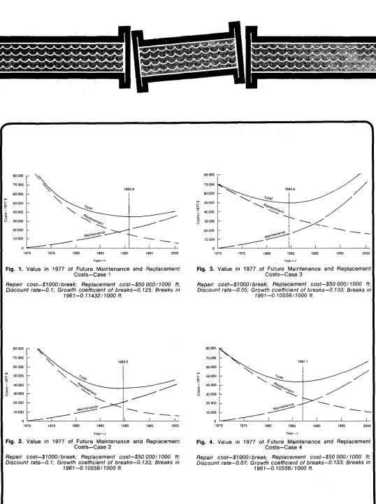
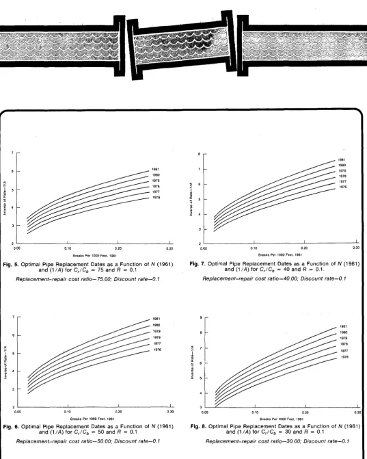
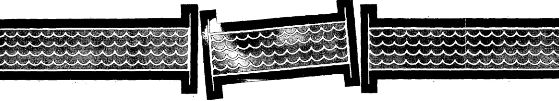
(3) form of the equation which forecasts the number of breaks in the existing and the new pipe. Appendix 1 analyzes the cases in which the new pipe has no future breaks or the same break history as the existing pipe, starting from an initial value appropriate for a new pipe. Economic Analysis and Results The economic analysis uses the following basic components: 1. The forecasted number of breaks in future years in the existing pipe 2. The forecasted number of breaks in the new pipe, as a function of the time from its installation 3. The cost of repairing one break 4. The cost of replacing the existing pipe with a new one 5. The discount rate which should be used in converting future expenditures into present value. The costs are expressed in today's dollars. Future expenses expressed in today's dollars can then be discounted, considering inflation, by using a discount rate calculated from the interest rate normally involved in the utility's financing and the anticipated cost of inflation. Alternatively, the discount rate could be determined from a more complex analysis based on the rates that taxpayers would have to pay if the funds were not received from taxation and could be applied to alternative investments or consumption. This approach involves calculation of an opportunity cost rate. In the present example a discount rate of 10 percent was selected as a representative compromise between both approaches. (The details of this calcula tion are explained in Appendix 2.) Figures 1-10 .show the results of the economic analy sis based on data for a particular area of Calgary, Alta. The practice in Calgary is to purchase new pipes of very high quality, provided with a jacket and cathodic protection. Experience has shown that new pipes are then practically break-free; it was therefore assumed in this study that the new replacement pipes would be break-free. Each of the first four figures is for a different pipe, and contains 1. A curve which shows the present value of all future replacement costs [Eq (1-3)] as a function of the replacement year 2. A curve which shows the present value of replac ing the pipe [Eq (1-4)] as a function of the replacement year 3. A curve which is the sum of the two previous ones 4. The optimal year for replacement, as computed from Eq (1-8). 250. MANAGEMENT AND OPERATIONS. The rate coefficient for the increase in breaks over time [A in Eq (1-1)] was found from the analysis of actual pipe break data. It showed that a compounding effect was taking place as time went on i.e., the number of breaks seemed to be increasing exponential ly. The way in which rate coefficient accounts for this effect is similar to the way in which an interest rate determines the compounding of investments. In Fig. 1 and 2 the same economic data have been used for pipes with different failure histories. Because of this, the optimal replacement dates are slightly different. The pipe having the lower number of breaks in 1961 experienced a higher rate of increase in breaks and should therefore be replaced a year earlier, in 1989, as shown in Fig. 2. In these examples the high 0.1 discount rate tends to shift the optimal replacement date to the right and results in a relatively flat total cost curve after that date. This effect is better illustrated in Fig. 3 and 4 which show that the lower discount rates produce a more sharply defined optimum replacement date that is closer to the present. Application in the field. For field use it might, be convenient to have charts that can be consulted as specific breaks are found. The remaining figures were developed for this purpose, but to use them, the failure history of the specific run of pipe must already have been analyzed. For the particular pipe to be examined the appropriate chart should first be selected from Fig. 5-8 by estimating the relative value of replacement cost to repair cost. Then, using the values for the rate coefficient A and the number of breaks in the base year N(t0), a point can be plotted on the chart. If this point falls below the curve representing the current year, the pipe should be replaced rather than repaired. If neces sary, a conclusion can be reached by interpolating from one chart to another. These charts can be easily prepared using the equa tion in Appendix 1, and a manual can be developed that would be applicable to all practical ranges of the various parameters. For example, if the replacement cost is $50 000 and the repair cost is $1000, their ratio is 50. Figure 5 shows that the optimal replacement year is 1980 for a pipe with a rate coefficient of 0.2 (I/A = 5) and approxi mately 1.25 breaks per mile (0.15/1000 ft) in the base year 1961. If replacement costs become still higher relative to repair costs, the optimal replacement data would be after the year 1980. However, as shown in Fig. 1-4, the total cost curves drop rapidly to a long shallow minimum and suggest that replacing a pipe too early is more costly than replacing it later than the optimal date JOURNAL AWWA.

(4) Fig. 1. Value in 1977 of Future Maintenance and Replacement Costs—Case 1. Fig. 3. Value in 1977 of Future Maintenance and Replacement Costs-Case 3. Repair cost—$1000/break; Replacement cost—$50 000/1000 ft; Discount rate—0.1; Growth coefficient of breaks—0.125; Breaks in. Repair cost—$1000/break; Replacement cost-$50 000/1000 ft; Discount rate—0.05; Growth coefficient of breaks—0.133; Breaks in. 1961-0.11432/1000 ft.. 1961-0.10556/1000 ft.. 80000 70000 60000 50000 40000 30000 20000 10000. 1985. 1990. 1980. 1985. Fig. 2. Value in 1977 of Future Maintenance and Replacement Costs—Case 2. Fig. 4. Value in 1977 of Future Maintenance and Replacement Costs—Case 4. Repair cost—$1000/break; Replacement cost—$50 000/1000 ft; Discount rate—0.1; Growth coefficient of breaks—0.133; Breaks in 1961-0.10556/1000 ft.. Repair cost—$1000/break; Replacement cost—$50 000/ WOO ft; Discount rate—0.07; Growth coefficient of breaks—0.133; Breaks in 1961-0.10556/1000 ft.. MAY 1979. U. SHAMIR & C.D.D. HOWARD. 251.

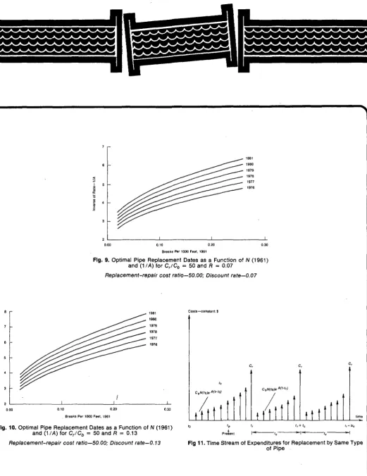
(5) suggested by the analysis. If the data used in the analysis are in doubt, it might be advisable to concen trate on repair rather than renewals. The effect of changing the discount rate is shown in Fig. 6, 9, and 10 for Cr/Cb = 50. Other applications. The relative proximity of the opti mal replacement time curves of Fig. 5-10 points to a high sensitivity of the results to the values of the various parameters. This is also demonstrated in the mathematical sensitivity analysis included in Appen dix 1. It may seem that this relatively high sensitivity to parameter values that cannot be accurately determined detracts from the usefulness of the results. This need not be the case because of the way in which the analysis can be used in practice. Frequently, perhaps every year, the analysis could be run for all the pipes in the network, using up-to-date data on breaks and considering current economic fac tors. This is possible because the analysis is so simple and inexpensive (although the difficulties and costs of mobilization for performing the analysis the first time may not be insignificant). The results can then be used in two ways: (1) to make a list of all pipes which according to the analysis should be replaced within the coming year; and (2) to make a list of pipe proposed for replacement in each of the coming, say, five years. The first list essentially separates all pipes in the network into two categories. In one category are pipes for which the optimal replacement time is the current year. (This includes pipes for which the replacement date is past; i.e., they should have already been replaced before the current year.) In the other category are all the pipes that need not be replaced immediately and can be analyzed in the next year, possibly with better data. The immediate concern is for those pipes that should be replaced in the current year. The list of these pipes can then be subjected to additional evalua tion considering factors such as the availability of funds, the necessary work force, and the effects of the replacement work on service. This amended list now gives the priority rating for replacement. The actual replacement list is therefore prepared after all the practical aspects have been considered. Pipes in the proposed list that are not replaced in the current year would be investigated again in the following year. The second list, that for each of the following few years, can be used in budgeting and planning funds and working teams for longer than just the current year. Although details may change in subsequent years as the analysis is repeated with new data, the current results are nevertheless useful for planning. 252. MANAGEMENT AND OPERATIONS. Effect of failures in new pipes. Appendix 1 includes an analysis conducted under the assumption that the new pipe will have the same history of breaks as the existing one. The same type of economic analysis could be carried out for other forms of the equation that describe the rate of change of breaks with time in the new pipe. From the numerical results presented in Appendix 1, it can be seen that projected future breaks in the new pipe have a relatively small effect on determining the optimal replacement time (for the typical parameter values used here). The reason for this is probably the rather high 0.1 discount rate used for the example. Conclusion. The economic analysis developed here is simple to calculate and can be programmed for a handheld calculator. The data required to develop realistic results may include a number of judgment factors related to repair and replacement costs, future interest and inflation rates, and anticipated failure rates in specified pipes. The analysis is therefore not a substi tute for good judgment, but it does provide a frame work within which good decisions can be made. Bibliography HANKE, S.H.; CARVER, P.H.; & BUGG, P. Project Evaluation During Inflation. Water Resources Res., 11:4:511 (Aug. 1975). JENKINS, G.P. The Measurement of Rates of Return and Taxation from Private Capital in Canada. Benefit-Cost and Policy Analysis (W. A. Niskanen et al, editors). Aldine Atherton, Chicago (1973). STOCKFISCH, J.A. Measuring the Opportunity Cost of Government Investments. Res. Paper P-490. Inst. of Defense Analysis, Arling ton, Va. (1969). Discount Rates to be Used in Calculating Time Distributed Costs and Benefits. OMB Circular A-94. US Ofce. Management and Budget, Washington, D.C. (Mar. 6, 1972).. Appendix 1: Timing of Replacement-Economic Analysis Pipe break data for a single pipe, several pipes with similar characteristics, or a whole region of the network are used to develop a regression equation for the number of breaks per year, N(i). A form that was found to fit well the data in one study is N(t) =' N(t,,)eA(<-i»). (1-1). where t = time in years, t0 = base year for the analysis (the year the pipe was installed, or the first year for which data are available) N(t) = number of breaks per 1000-ft length of pipe in year t JOURNAL AWWA.

(6) 0.00. 0.20. 0.10. 0.10. 0.20 Breaks Per 1000 Feet, 1961. Breaks Per 1000 Feet, 1961. Fig. 5. Optimal Pipe Replacement Dates as a Function of W (1961) and (1 XXI) for Cr/Cb = 75 and R = 0.1. Fig. 7. Optimal Pipe Replacement Dates as a Function of N (1961) and (1 /A) for Cr/Cb = 40 and R = 0.1.. Replacement-repair cost ratio—75.00; Discount rate—0.1. Replacement-repair cost ratio—40.00; Discount rate—0.1. 0.20. 0.10 Breaks Per 1000 Feet. 1961. Fig. 6. Optimal Pipe Replacement Dates as a Function of W (1961) and (1//4) for Cr/Cb = 50 and R = 0.1 Replacement-repair cost ratio—50.00; Discount rate—0.1. MAY 1979. 0.10. 0.20 Breaks Per 1000 Feet, 1961. Fig. 8. Optimal Pipe Replacement Dates as a Function of N (1961) and (1/Xl) for Cr/Cb = 30 and R = 0.1 Replacement-repair cost ratio—30.00; Discount rate—0.1. U. SHAMIR & C.D.D. HOWARD. 253.

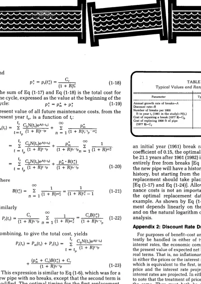
(7) A = growth rate coefficient (dimension is I/ year). In this study, conducted in 1976-77, the rate coefficients were found to range between 0.05-0.15. This means that the number of breaks will double in a period between 4.6 and 13.8 years. The year 1961 was used as the base year for Eq (1-1), with values of N(t0) ranging between 0.10 and 0.25 breaks/1000 ft/year. Equation (1-1) will be used in the economic analysis. It should be noted that the economic analysis can be carried out in a similar fashion, if a linear or polynom ial form of growth equation is found to fit the data better. We shall later investigate the sensitivity of the results of the economic analysis to values of the parameters in Eq (1-1). As the number of breaks per year increases, so does the cost of repairing them. If the cost of repairing a break Cb, expressed in constant dollars, is assumed to be constant over time, then the cost of repairing the breaks in 1000 ft of the pipe in the future year t is (1-2) Cm(t) = CbN(t) = CbN(t,,)eA«-'o) If the present year is denoted by tp , and the (noninflationary) discount rate is R, then the present value of this maintenance cost is simply Cm(f) (1-3) R)t-'P Denote by tr the year in which the pipe will be replaced. The present value of all maintenance cost from the present year tp to the year tr for 1000 ft of pipe is. tr If the new pipe will not incur any breaks, then Pm (tr) represents all future maintenance costs. Other cases will be discussed later. The cost of replacing 1000 ft of pipe, expressed in the same constant dollars as Cb , is Cr. The present value in year tp of replacing 1000 ft of pipe in year tr is therefore. cr R)tr'lp. (1-5). Pm (tr) is an increasing function of tr, because for every additional year that passes before the pipe is replaced there is an additional term in Eq (1-4). On the other hand, Pr(tr) decreases with tr because it is assumed that 254. MANAGEMENT AND OPERATIONS. Cr is constant, whereas the denominator increases with t,-. The optimal timing for replacement is that year for which the total cost. PrM - PJU + PM - J (T^ i IP is a minimum. We thus seek that value of tr, denoted t*, which minimizes Eq (1-6), i.e., Cr. MinT ' *r L t1 = ,. Differentiating with respect to tr, setting equal to zero, and solving, we get the optimal value A. (1-8). N(QCh. This result holds for t* < tp (i.e., the optimal year is in the past), as well as for t* > tp, even though the denominators in Eq (1-7) have no economic meaning when t* < L. The reason is that the denominators vanish in solving for t*. The base year t0 used in developing the regression Eq (1-1) has no influence on the solution. This can be seen by observing that the number of breaks at some other year, say the present year tp , is, from Eq (1-1) N(tp) = WftJe'V'p W and therefore, for any future year t N(t) = = N(tPVC~'p) Thus, Eq (1-4) can be written tr CM ft ) • b ( v' (t ) = v P m(r). (1-1.1). (1-4.1). Introducing this expression into Eq (1-7), differentiat ing, setting equal to zero, and solving for t* leads to A. N(tfy). This expression gives the same results as Eq (1-8), demonstrating that the arbitrarily selected base year t0 has no effect on the result. Table 1 contains typical values of the various paramJOURNAL AWWA.

(8) 0.20. 0.10 Breaks Per 1000 Feet, 1961. Fig. 9. Optimal Pipe Replacement Dates as a Function of N (1961) and (1 /A) for Cr/Cb = 50 and R = 0.07 Replacement-repair cost ratio—50.00; Discount rate—0.07. Costs—constant $. 0.20. 0.10 Breaks Per 1000 Feet, 1961. Fig. 10. Optimal Pipe Replacement Dates as a Function of N (1961) and (1A4) for Cr/Cb = 50 and R = 0.13 Replacement-repair cost ratio—50.00; Discount rate—0.13. MAY 1979. ill. lit. 111. Present. Fig 11. Time Stream of Expenditures for Replacement by Same Type of Pipe. U. SHAMIR & C.D.D. HOWARD. 255.

(9) eters resulting from the study in Calgary, Alta. Using the typical values in Eq (1-8) yields t* = t0 + 77.3; i.e., the pipe is to be replaced 77 years after the base year t0. For A = 0.10, all other data remaining the same, t* = t0 + 38.6. Figures 1-4 in the paper show the shape of the total , cost PT and its two components, Pm and Pr. The optimal timing for replacement t*, which is at the minimum of PT, corresponds to the year in which the annual increase in Pm is just equal to the annual decrease in P, If the increase in breaks were linear, and given by NftJ = N(t0) A (t-g (1-9) then the optimal timing for replacement would be given. by. t* = t» +. R) Cr A N(t0) Cb. (1-10). Equation (1-8) is the basis for the results presented throughout this paper, because Eq (1-1) was found to fit well the data we have analyzed. The sensitivity of t* to variations in parameter values is obtained by differen tiating Eq (1-8) with respect to each parameter. ill = =1 ln fln(l + R) Cr"[ a3 A ^ L N(t0) Cb -I. (1-11). 3 1; _. (1-12). a R. i. A(l + R) ln(l + R). a t* _ -l a N(t,,) AN(t(1). (1-13). a t; _ -l a Cb ACb. (1-14). a Cr. (1-15). ACr. To gain an appreciation of these sensitivities we shall use the typical values of the parameters as given in Table 1. The results are. _£_*!= -1565 3 A. t* will decrease by one year for an increase of 0.00064 in A, or by 15.6 years for an increase of 0.01 in A.. . = 200. t* will increase by one year for an increase of 0.5 percent in R, or by two years for a 1 percent increase in R.. 3 R. 256. MANAGEMENT AND OPERATIONS. 3 t*. d N(to). = 200 t* will decrease by one year for an increase of 0.005 in N(t0).. d t*. - = 0.02 dCb. t* will decrease by one year for an increase of $50 in Cb.. = 0.0004. t* will increase by one year for an increase of $2500 in Cr. These are the sensitivities to a change in one param eter at a time, all other parameters being at their typical values. Effect of breaks in the new pipe. All the above results were for the case in which the new pipe will experience no breaks. Next, we examine what happens when the new pipe is expected to have breaks, but at an initial rate which is lower than the current rate in existing pipe. (If it were not lower there would be no reason for replacement.) An economic analysis can be carried out for any assumed rate of breaks in the new pipe. We shall analyze, as an example, the case in which the new pipe is the same type as the existing one and, once in stalled, will have the same future history of breaks as the old one had in the past. We shall assume that the number of breaks will start at N(t0) and increase at a rate given by Eq (1-1) with the same rate coefficient A. Figure 11 depicts the stream of future expenditures for this situation. The pipe presently in service is to be replaced in year tr, at a cost of Cr ($71000 ft). Once installed, the new pipe will experience breaks at a rate given by Eq (1-1), and therefore the stream of mainte nance costs is given by Eq (1-2). Following the first replacement the pipe will be replaced every tc years. The length of the optimal replacement cycle, t*, is given by Eq (1-8), i.e., » = _L In Fln(1 + ft) Cr1 tc A L N(t0) Cb J t1 - 16) a Cr. This is because the end of the cycle is such that the annual increase in total maintenance cost Pm (present valued to tr or to tp , it makes no difference to the result) is just equal to the annual decrease in total replacement cost Pr. Each cycle is therefore balanced in itself. It is then necessary to define for each cycle the costs of maintenance and replacement, expressed in their value at the beginning of the cycle. For the optimal cycle length, t*, these are P = PmO*) =. 2 t = 1 (1 +. (1-17). which is easily programmed for a hand calculator, JOURNAL AWWA.

(10) and TABLE 1 Typical Values and Ranges for Parameters. Pi = Pr('c) =. The sum of Eq (1-17) and Eq (1-18) is the total cost for one cycle, expressed as the value at the beginning of the cycle: p* = p* + p* (1-19) Present value of all future maintenance costs, from the present year tp , is a function of tr : P in - y CbN(t,)e*ft-t.J °° P* rm(tr) - —2, | I, -I "T" II1 p. r + — 2.— -1 (l~r ft If n C tn. '. 11. R)'-tp. =. £ CbN(t0)e'M'-'o) + t =. j.. '. 2 n = i (1 +. H)''-'Pn = B(t*) R)tr-lp. (1-20). (1 + R)'* -. (1-21). Similarly «)''-'». R)'r-lp n =. Typical Value. Range. 0.05 0.10 0.10. 0.01-0.15. 1000 50000. 500-2000 10 000-150 000. 0.05-0.15 0.01-0.20. r. where B(t*) =. Parameter Annual growth rate of breaks A Discount rate R Number of breaks per 1000 ft in year t. (1961 in the study)-N(t,,) Cost of repairing a break (1977 $} C b Cost of replacing 1000 ft of pipe (1977 $)-Cr. (1-22). an initial year (1961) break rate of 0.2, and a growth coefficient of 0.15, the optimal replacement time would be 21.1 years after 1961 (1982) if the new pipe were to be entirely free from breaks [Eq (1-8)]. If future breaks in the new pipe will have a history similar to the old pipe's history, but starting from the date of replacement, the replacement should take place one year later, in 1983 [Eq (1-17) and Eq (1-24)]. Allowance for future mainte nance costs is not an important factor in determining the optimal replacement date, at least not for the example. As shown by Eq (1-24), the time to replace ment depends linearly on the inverse rate coefficient and on the natural logarithm of the other factors in the analysis. Appendix 2: Discount Rate During Inflation. Combining, to give the total cost, yields t. P|(t,) = Pm(tr) + PA) =. 2. ^^. t = tp (1 + H)'-'p. , (p* + Cr)B(t*) + Cr (1 + R)'r-tp. (1-23). This expression is similar to Eq (1-6), which was for a new pipe with no breaks, except that the second term is modified. The optimal timing for the first replacement, t*, is given by an expression similar to Eq (1-8), namely. ct ]I] (1-24) A "L N(t.)Cb This expression is similar to Eq (1-8), which was for a new pipe which has no future breaks. Now, however, the second term contains the factor (Cr + p^,) B(t*) which accounts for the future cycles of replacement and maintenance. As an example, using a discount rate of 0.1, replace ment and repair costs of $50 000 and $1000 respectively, t; - t. + JL inpfi- R)[(Cr. MAY 1979. For purposes of benefit-cost analysis, inflation can consis tently be handled in either of two ways. First, prices and interest rates, the economic components used in computing the present value of expected net benefits, can be projected in real terms. That is, no inflationary components are included in either the prices or the interest rates. The second approach, which is equivalent to the first, includes inflation in both the price and the interest rate projections; nominal prices and interest rates are projected. In either approach it is important to note that the treatment of prices and interest rates must be the same. They must both be projected in either real or nominal terms. (Hanke et al, p. 512).. The approach used here is to work with the real costs and a real, inflation-free, discount rate R. To calculate the appropriate discount rate it is necessary to develop its relationship to the more readily available market rate of interest r, using the expected rate of price change as reflected in the inflation rate I. At the end of a particular time period the value of db dollars invested at the real rate of interest R at the beginning of the time period would be Ce, given by Ce = db (l + R) (2-1) U. SHAMIR & C.D.D. HOWARD. 257.

(11) If inflation is involved, the final amount de would need to be even greater if the purchasing power of the original amount db is to be preserved. Thus de = db (l + R) (1 + I). (2-2). The nominal interest rate r gives the same final amount for the same initial investment, i.e., de = db (1 + r) Equating (2-2) and (2-3), (1 + r) = (1 + R) (1 + I) from which, r-I R 1-f. (2-3) (2-4). (2-5). in which r = the nominal (market) rate of interest I = the inflation rate for water main projects R = the real (inflation-free) rate of interest to be used in present value computations for water main projects. The values of the market rate of interest and the inflation rate could in principle be estimated for each interval, making them a function of time. Here both r and I have been assumed to be constant over the time period of interest. The present value factor at year tp , of a discrete series of time increments from tp to tn , is then given by (2-6). During a period of high inflation a continuous repre sentation may be more appropriate. In this case let er ' = (1 + rd)>. (2-7). in which rc is the continuous market rate of interest and rd is the discrete rate, used in Eq (2-5). Their relation ship is therefore given by rc = ln(l -I- rd). (2-8). Carrying out the analysis again for the continuous case, equations analogous to Eq (2-l)-(2-4) lead to Rc = rc -lc. (2-9). in which the subscript c indicates that continuous values are to be used. For the analysis of Appendix 1, Eq (2-5) is used. 258. MANAGEMENT AND OPERATIONS. Alternatively the optimal replacement time and the other equations could be derived using e- Kc'as a present value factor in place of (l + Rd)^. The selection of an appropriate discount rate for public investment could be made on the basis of an opportunity cost calculation which considers alterna tive uses of funds, as well as relative prices within the economy and their relative rates of inflation. For public projects, financed by taxes, such an analysis would have to consider the alternative uses which taxpayers might have for their money other public projects, advance payments on a house mortgage, cash instead of terms for automobile and appliance purchases, or investments in various securities are all possibilities. Such considerations form the basis of an opportunity cost rate for public projects. This rate is, in effect, some meaningful weighted discount rate that the taxpayers might recognize as personally meaningful. Hanke et al derive the correct relationship between the real and nominal interest rates and discuss the two ways in which the real interest rate can be computed. They proceed to criticize the Water Resources Develop ment Act passed by the US Congress in 1974, according to which real prices and nominal interest rates are to be used, and conclude by saying: To correct this error, we recommend: (1) that real prices (which appropriately account for changes in relative prices) should be projected for undiscounted expected benefits and costs; and (2) that real interest rates (preferably the real social opportunity cost rather than the real financial cost) should be used to discount these values. This would mean that the interest rate to be used in conjunction with real prices should not be the recommended 'Adjusted nominal financial rate' (5% percent) or the real financial rate (4 percent) but the real opportunity cost rate. The weighted average real opportunity cost rate, as calculated by Stockfisch (1969), is approximately 10.4 percent. It is interesting to note that Jenkins (1973) in a comparable study has calculated this rate to be 9.5 percent for Canada. It is also interesting to note that the US Office of Management and Budget (1972) recommended that a 10 percent rate be used for evaluating most federal investment decisions, including those for water resource projects. Unfor tunately, their recommendations have not been adopted in the water field.. In the study reported here, real prices were used and the real interest rate taken to be 10 percent. A paper contributed to and selected by the JOURNAL, authored by Uri Shamir, dir., and Charles D.D. Howard (Active Member, AWWA), pres., both of Charles Howard & Assoc., Ltd., Winnipeg, Manitoba, 55585. 5600 JOURNAL AWWA.

(12)

No results found