i
Methods for Analyzing the Information Content of
Large Neuronal Populations
by
Palipahana Pahalawaththage Chamanthi Rasangika Karunasekara
First Supervisor: Prof Stefano Panzeri
Second Supervisor: Dr Arno Onken
Submitted to Center for Mind/Brain Sciences (CIMeC)
in Partial Fulfillment of the Requirements for the Degree of
Doctor of Philosophy
at the
University of Trento
ii
ABSTRACT
iii
ACKNOWLEDGEMENTS
This work would not have been possible without the support of many people. I would like to thank my primary advisor Prof. Stefano Panzeri, who always believed in me and encouraged me throughout these years. I would also like to thank Dr. Arno Onken, my second advisor, for the encouragement and collaboration during the years. The data used in this thesis include those that were kindly provided to us by Shuzo Sakata and collaborators at Strathclyde University and Tim Gollisch and colleagues from University of Gottingen. Ioannis Delis from Columbia University collaborated with us on our algorithms. I owe much gratitude to the Marie Curie Initial Training Network, Adaptive Brain Computations (ABC, grant agreement number PITN-GA-2011-290011) that supported my work. I gained much insight from the workshops, lab visits and meetings that took place and I was fortunate to be part of diverse and collaborative research community. I thank everyone in our Neural computation lab. I am very grateful to be part of our group. Many people including Sara Maistrelli, Paola Battistoni and Leah Mercanti helped and advised me in many administrative matters. I would also like to thank all my colleagues and other personnel in IIT, CIMeC and University of Trento with whom I got the opportunity to work and share experience with, who have assisted me and who were good to me in various ways during the years.
iv
TABLE OF CONTENT
ABSTRACT ... II ACKNOWLEDGEMENTS ... III LIST OF FIGURES ... VI LIST OF TABLES ... VII
CHAPTER 1: INTRODUCTION... 8
1.1THE BRAIN AS AN INFORMATION PROCESSING MACHINE ... 9
1.2BRAIN STATES ... 10
1.3NEURAL POPULATION CODES ... 11
1.4NEURAL CORRELATIONS ... 15
1.5METHODS TO ANALYZE NEURAL POPULATIONS ... 17
1.5.1 Statistical methods ... 18
1.5.2 Model-based methods ... 18
1.5.3 Decoding ... 20
1.5.4 Mutual information ... 21
1.5.5 Dimensionality reduction methods ... 23
1.6OVERVIEW OF THE THESIS ... 31
CHAPTER 2: NON-NEGATIVE MATRIX FACTORIZATION TO EXTRACT SPATIOTEMPORAL SPIKE PATTERNS ... 33
2.1ABSTRACT ... 33
2.2INTRODUCTION ... 33
2.3NON-NEGATIVE MATRIX FACTORIZATION... 35
2.4NMF FOR SPATIOTEMPORAL SPIKE ACTIVITY ... 36
2.5REPRESENTATION OF SPATIOTEMPORAL NEURAL RESPONSES USING NMF ... 41
2.5.1 Using NMF to study population coding of sounds in rat auditory cortex ... 41
2.5.2 Using NMF to study population coding of stimulus location in rat somatosensory cortex... 52
2.5.3 Using NMF to study encoding of visual information by populations of retinal ganglion cells ... 59
2.6DISCUSSION... 68
CHAPTER 3: EXTENSION OF SPACE-BY-TIME NMF TO MODEL VARIABILITY IN NEURAL SPIKE TRAINS ... 70
3.1ABSTRACT ... 70
3.2INTRODUCTION ... 70
3.3EXTENSION OF SPACE-BY-TIME NMF ... 71
3.3.1 Dissimilarity measures used in NMF ... 72
3.3.2 NMF as a generative model ... 73
3.3.3 Noise models for neural variability... 74
3.3.4 Bregman divergences to model neural variability ... 75
3.3.5 Update rules for space-by-time NMF that model neural variability ... 77
3.4PERFORMANCE EVALUATION ... 82
3.4.1 Statistical simulations ... 82
3.4.2 Network simulations ... 86
3.4.3 Using new update rules to study population coding of sounds in rat auditory cortex ... 94
v
3.5DISCUSSION... 111
CHAPTER 4: DISCUSSION ... 115
4.1NMF WITH RESPECT TO OTHER METHODS THAT CAN BE USED TO STUDY SPATIOTEMPORAL ACTIVITY ... 115
4.2BACKGROUND OF NMF AS A METHOD TO STUDY POPULATION ACTIVITY ... 116
4.3MODELING NEURAL VARIABILITY USING SPACE-BY-TIME NMF ... 117
4.4EFFECT OF OUTLIERS ... 118
4.5SPACE-BY-TIME NMF TO STUDY POPULATION CODING IN SPACE AND TIME ... 119
4.6FUTURE DIRECTIONS ... 122
APPENDIX 1: PROOF OF THE EQUIVALENCE OF MINIMIZATION OF THE BREGMAN DIVERGENCE AND THE MAXIMUM LIKELIHOOD ESTIMATION OF THE MEAN FOR BINOMIAL AND NEGATIVE BINOMIAL UPDATE RULES ... 123
APPENDIX 2: CHANGES IN RESPONSE PROPERTIES OF AUDITORY CORTICAL NEURONS TO STATE CHANGE... 126
vi
LIST OF FIGURES
Figure 1.1: Coding of the movement direction using average firing rates ... 13
Figure 1.2: Illustration of latency code as an example of a spike timing code. ... 14
Figure 1.3: Illustration of spatiotemporal trajectories coding stimuli. ... 15
Figure 1.4: Information limiting correlations ... 16
Figure 1.5: Illustration of the generalized linear model (GLM) for two neuron network. ... 19
Figure 1.6: Illustration of extending mutual information (MI) to larger populations using a decoding framework. ... 22
Figure 1.7: Principal component analysis (PCA). ... 24
Figure 1.8: State transition diagram for a model with three hidden states. ... 29
Figure 2.1: Illustration of two-factor NMF applied on a facial image dataset and the reconstruction of an image using underlying modules... 37
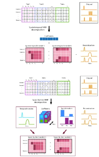
Figure 2.2: Illustration of spatiotemporal NMF and space-by-time NMF models. ... 38
Figure 2.3:Space-by-time module structure for responses of 85 A1 neurons to click sequences. ... 44
Figure 2.4: Changes observed in the neural responses of auditory neurons between the two levels of synchronization. ... 47
Figure 2.5: Space-by-time module structure for responses of 85 A1 neurons to long tones. ... 50
Figure 2.6: Stimulus discrimination capability of the low-dimensional representations extracted by NMF. ... 51
Figure 2.7: Module structure and the decoding performance of spatiotemporal NMF and space-by-time NMF on the response of 300 neurons to whisker deflections. ... 54
Figure 2.8: Reconstruction of population responses using space-by-time NMF ... 56
Figure 2.9: Analysis of neural responses of 49 retinal ganglion cells for flashed natural images. ... 62
Figure 2.10: Analysis of neural responses of 54 retinal ganglion cells for full-field gratings. ... 63
Figure 2.11: Analysis of neural responses to shifted natural images. ... 64
Figure 3.1: Illustration of space-by-time NMF under different noise models. ... 72
Figure 3.2: Performance evaluation of new update rules using statistical simulations. ... 83
Figure 3.3: Conductance-based integrate and fire network simulations. ... 87
Figure 3.4: Simulation of network responses to long tones. ... 91
Figure 3.5: Variation of the weights of neurons in the spatial modules (SM) with the mean firing rates. ... 92
Figure 3.6: The module structure derived from Gaussian and Poisson space-by-time NMF rules for the neural responses recorded from 85 A1 neurons to long tones. ... 96
Figure 3.7: The module structure derived from Gaussian and Poisson space-by-time NMF rules for the neural responses recorded from 85 A1 neurons to click sequences. ... 97
Figure 3.8: Decoding performance of auditory responses using space-by-time NMF rules. ... 98
Figure 3.9: Analysis of first spike latency. ... 101
Figure 3.10: Spatial modules identified by space-by-time NMF for spike latency analysis. ... 102
Figure 3.11: The performance of space-by-time NMF update rules after preprocessing data. ... 103
Figure 3.12: Application of space-by-time update rules on trial-shuffled responses to long tones and click sequences... 104
Figure 3.13: Module structure and the coefficients extracted by Gaussian and Poisson update rules from the neural responses of 300 neurons to whisker deflections ... 109
vii
LIST OF TABLES
8
Chapter 1:
Introduction
Neural populations from sensory areas (Stopfer et al., 2003; Jones et al., 2007), motor areas (Churchland et al., 2012) to higher level regions (Durstewitz et al., 2010; Mante et al., 2013) exhibit collective dynamics in response to stimuli. Neural population activity can be characterized using two dimensions; space and time. The spatial dimension describes how neurons modulate their tuning and interactions to represent stimuli (Rigotti et al., 2013; Moreno-Bote et al., 2014; Panzeri et al., 2015; Pitkow et al., 2015). The temporal dimension describes how the collective activity of a population of neurons evolves over time, which can contain information that is lost if the fine details of the population activity across time is neglected.(Laurent, 1999; Petersen et al., 2002; Stopfer et al., 2003; Heil, 2004; Gollisch and Meister, 2008; Panzeri et al., 2010a; Zuo et al., 2015). With the recent advancements in recording methods it is now possible to record from hundreds of neurons simultaneously (Buzsáki et al., 2015). An emergent view from the insights gained from these large scale recordings is that the neural population activity consists of a limited number of stereotyped spiking patterns (Nádasdy et al., 1999). Sometimes these groups of neurons tend to fire close together in time, with the relative strength and timing of recruitment of different patterns encoding information about the stimulus features (Luczak et al., 2009; Luczak et al., 2013).
How to extract a biologically meaningful and scalable representation of neural population spike trains in space and time remains an open problem. The purpose of this thesis is to make a contribution towards finding mathematical methods that can accomplish this goal. When developing such a method, first one has to identify the key requirements that the derived representation has to fulfill. It should satisfy many requirements. First, because the brain makes decisions in single trials, it should capture information in single trial spike trains. Second, it should capture most or all information about stimuli with a small number of parameters. Third, the basis functions used to describe single-trial neural activity should be interpretable biologically: in particular, it should decompose neural activity into the constituent stereotyped patterns of firing observed in the data..
Current methods for finding low-dimensional representations of neural activity (Laubach et al., 1999a; Byron et al., 2009; Yu et al., 2009; Churchland et al., 2010; Cunningham and Byron, 2014) such as Principal Component Analysis (PCA), Independent Component Analysis (ICA), or Factor Analysis (FA) are usually applied to firing rate only, neglecting the temporal structure of spike trains, or to trial-averaged data in order to avoid the confounding effects of trial-to-trial spiking.
9
advantages: its basis functions and coefficients are, in principle, interpretable as firing patterns and as their strength of recruitment in single trials; it generates sparse representations; and it can cope with non-orthogonal firing patterns such as the partly overlapping ones that may be generated by neural circuits with hard-wired connectivity.
In this thesis we will explore in detail the potentials of NMF for spike train analysis by studying carefully the mathematical basis for application to spike trains such as assumptions to be made regarding the spatial and temporal nature of neural responses, models or neural noise or neural variability. We introduce and refine NMF based methodologies to study population coding that address the above mentioned key requirements. We apply it systematically to many different datasets of neural responses.
Before I proceed further in studying these topics, in this introductory chapter I will review some basic empirical facts of neural population coding and some of the techniques currently used to study it. I will conclude with an overview of the other chapters of this thesis.
1.1
The brain as an information processing machine
The brain is an information-processing machine. It constructs representations of the external world from signals coming from our sensory organs. Computations on these representations lead to the way we perceive the world, remember past events, plan our future and make day-to-day decisions. Our actions and behaviors in turn are initiated from signals that our brain sends to our motor elements (Decharms and Zador, 2000). The fundamental question in neuroscience is to understand how our brain performs these functions.
Neurons are the basic information processing units in the brain. A neuron participates in information processing through changes in its membrane potential. Its membrane potential is generally at a resting value, but can change in a transient stereotypical voltage profile generating an action potential or a spike. Neurons communicate with each other by transmitting action potentials across chemical or electrical synapses. Typically, a neuron receives about 3000 - 10000 pre-synaptic connections from which about 85% are excitatory and the remaining are inhibitory (Mayhew, 1991; Shadlen and Newsome, 1998). Excitatory pre-synaptic spikes cause an increase in the membrane voltage of an excitatory neuron while inhibitory pre-synaptic spikes cause a decrease in its membrane voltage. Even though a neuron receives a large amount of inputs with strong temporal fluctuations, a neuron typically maintains a reasonably low firing rate with variable spike times through a balance in excitation and inhibition (van Vreeswijk and Sompolinsky, 1996; Shadlen and Newsome, 1998; Wehr and Zador, 2003; Okun and Lampl, 2008).
10
from afferent thalamocortical connections. Layer V cells connect cortex to sub-cortical structures such as basal ganglia, while neurons in layer VI send efferent connections to the thalamus. In the columnar organization, a column is a vertical cluster of neurons that have similar functional roles (Mountcastle et al., 1957; Mountcastle, 1997). An example is a barrel column in rodent somatosensory cortex where inputs from the thalamus relating to a single whisker terminate at a distinct area in the layer IV of the somatosensory cortex called barrel column (Woolsey and Van der Loos, 1970). The number of neurons per column varies with the distance of the respective whisker from the ground (Meyer et al., 2013). Another example is the columnar organization found in V1 that is defined by the ocular dominance and the orientation specificity (Hubel and Wiesel, 1959, 1962; Obermayer and Blasdel, 1993). While a similar architecture is found in many other cortical regions (Mountcastle, 1997), the reasons for the existence of such columnar organization is debated (Horton and Adams, 2005).
Experimental studies have found that neuronal connectivity can be highly clustered and neurons can form sub-networks at a fine-scale (Song et al., 2005; Yoshimura and Callaway, 2005; Yoshimura et al., 2005; Perin et al., 2011). The synaptic weight that specifies the strength of the connection between the pre-synaptic neuron and the post-synaptic neuron could be strong in a few synaptic connections that are more clustered (Song et al., 2005). Interconnected sub-networks could also share a higher degree of common excitatory input (Yoshimura et al., 2005) and process related sensory information with high functional specificity (Ko et al., 2011). Such sub-networks define localized organization at a finer scale within the cortex, which can give rise to coactivations and interactions between clustered neurons. Recent studies have proposed that the population activity is constrained to display stereotypical activity patterns that are recruited to encode sensory stimuli and to coordinate motor activity (Luczak et al., 2009; Sadtler et al., 2014).
1.2
Brain states
11
synchronized and a highly desynchronized state. Mechanisms such as attention can cause changes in neuromodulation that result in changes of the state of the brain at a local level (Harris and Thiele, 2011). Furthermore, when experiments are conducted under anesthesia such as urethane, spontaneous changes in the brain state could be observed (Clement et al., 2008; Curto et al., 2009). One of our datasets exhibits such a spontaneous state change. The state of the brain is relevant for sensory processing because the responses of neurons to external sensory inputs are shaped from the state of the cortex. Salient stimuli such as auditory clicks and whisker deflections generate large responses irrespective of the state of the brain while temporally extended stimuli are processed efficiently only in the desynchronized state (Harris and Thiele, 2011). Thus, there is a considerable influence of the endogenous brain state on the neural activity.
Scientists conduct experiments to understand how external stimuli are presented in the brain and how computations on these representations lead to cognitive functions and motor actions. Based on what we know of the structure of the brain, how it represents the outside world and performs computations, we record responses from a population of neurons in the brain region that we believe to be involved in the task that we wish to investigate. We look at the recorded activity and try to decipher how the recorded population of neurons modulates their spiking to perform the representation or the computation using a method suitable to analyze the recorded neural activity. We further explore how the states of the brain shape this activity in time. We will now look at some ways in which neurons are known to represent the external world, or more specifically, how they represent the set of stimuli we present during the experiment. Methods that are used to analyze neural activity, which we will discuss later, are designed to suit what we know of these representations.
1.3
Neural population codes
The set of response properties that carry information about the stimuli is called the neural population code (Panzeri et al., 2015). There are many features in the recorded population responses that can convey information about stimuli (Onken et al., 2014; Panzeri et al., 2015).
12
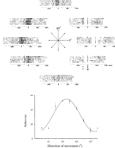
(Georgopoulos et al., 1982; Georgopoulos et al., 1983; Edelman et al., 1984) shown in Figure 1.1A shows the raster responses of a cell to five trials each recorded when a monkey made hand movements from a central position to the eight equi-spaced directions indicated at the center. The firing rate of the cell shown in the tuning curve in Figure 1.1B is clearly modulated to the movement direction and defines a rate code for movement direction. In higher cortical areas neurons show mixed selectivity to a range of task related parameters simultaneously (Rigotti et al., 2013). The selective modulation of the firing rate across a neural population is a form of stimulus coding across the spatial dimension.
13
Figure 1.1: Coding of the movement direction using average firing rates A: Raster plots of responses recorded from a neuron in the proximal motor area of a monkey when the hand was moved from a central position to the periphery in each of the eight directions indicated in the center. The movement is made after the target (T) is shown at the time indicated by longer vertical lines. Trials are aligned to the movement onset M also indicated by longer vertical bars. B: The tuning curve of the cell in A showing the average firing rate of the neuron for the eight directions (The image is in (Edelman et al., 1984) and was adapted from (Georgopoulos et al., 1982b))
A
Sp
ik
es/s
ec
14
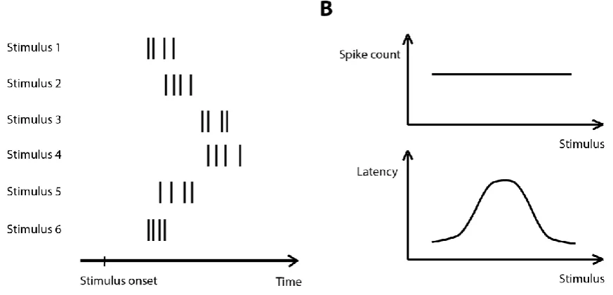
Figure 1.2: Illustration of latency code as an example of a spike timing code. A: Responses of a hypothetical neuron to six stimuli B: The tuning curves constructed using the spike counts of the cell (top) and the first spike latency (bottom).
When identifying neural codes that require the knowledge of either the stimulus onset or the segmentation of the response into informative bins, the natural question is how biologically realistic such a scheme could be. Is it possible for the brain to formulate this knowledge to use such a coding scheme? Some experimental studies have shown indications that such knowledge is available at the cellular level (Chase and Young, 2007; Onken et al., 2014; Panzeri et al., 2014). Subpopulations of neurons within the auditory cortex have been identified that respond early and reliably in a stimulus invariant way (Brasselet et al., 2012). When the response onsets of the remaining stimulus modulated neurons were set to the response onsets of these stereotyped neurons, about 95% of the spike timing information could be extracted indicating that this scheme could serve as a reliable way of identifying the stimulus onset. Similarly, in the somatosensory system, when single whiskers are deflected, the whisker position can be identified on a millisecond time scale by using the latency from the time at which a large portion of the neurons in the columns fired synchronously (Panzeri and Diamond, 2010). To address the question of how the brain could segment long time intervals into informative segments, (Kayser et al., 2009) indicated that when the spike train was partitioned into segments using the phase of the theta (2 - 6 Hz) frequency band in the local field potential forming a phase-partitioned code, it carried almost similar information as a time-partitioned code using the laboratory clock, which was large compared to information only in the total spike count. Finally, there is experimental evidence that timing codes could be read out from downstream neurons (Haddad et al., 2013; Uchida et al., 2014).
15
some form of dimensional reduction method is used to analyze and visualize this activity. Visualization is done in the space defined by the low-dimensional components (latent components). In the illustrative example shown in Figure 1.3, the activity of N neurons is represented in the 3-dimensional latent component space. Each stimulus evokes a different trajectory in this space. Thus, each stimulus is coded by a different pattern of population activity evolving in space and time.
Figure 1.3: Illustration of spatiotemporal trajectories coding stimuli. The high dimensional neural activity is visualized using a dimensionality reduction method in the three dimensional latent component space. Each stimulus evokes a different trajectory in the component space.
Collective behavior becomes increasingly important as the number of recorded neurons increases. As the size of the population becomes large, spikes of individual trials can be predicted more accurately using models based on pairwise interactions between neurons compared to models that predict spikes based on external stimuli (Stevenson and Kording, 2011). Thus, we next briefly look at the effects of correlated behavior in neural coding.
1.4
Neural correlations
16
(Abbott and Dayan, 1999; Sompolinsky et al., 2001; Wilke and Eurich, 2002; Shamir and Sompolinsky, 2006; Josic et al., 2009; Ecker et al., 2011; Moreno-Bote et al., 2014). When a population has similar tuning curves and has positive noise correlations, correlations limit the information coding capability (Sompolinsky et al., 2001), while such a limit does not exist when the neurons have heterogeneous tuning (Shamir and Sompolinsky, 2006). (Moreno-Bote et al., 2014) formulated that correlation structures that limit the level of information coding has a component in the covariance matrix that is proportional to the product of the derivatives of the population responses. An illustrative example from (Moreno-Bote et al., 2014) is shown in Figure 1.4. It shows the mean population activity f s( ) in the N-dimensional space. The distribution of the trial-to-trial variability is shown by the yellow curve. When this distribution has a small curvature along f s( ), it can be approximated with the blue distribution that lies on the tangent to the mean population response indicating that
the covariance matrix is proportional to ' T
f'f .
Correlational structures are not static. Experimental studies indicate that they can change dynamically with variations in attention and brain states (Steinmetz et al., 2000; Gutnisky and Dragoi, 2008; Cohen and Maunsell, 2009; Curto et al., 2009; Pachitariu et al., 2015). Certain correlation structures that show stimulus dependent changes can give substantial increases in the level of information coding (Franke et al., 2016; Zylberberg et al., 2016). Thus, noise correlations can shape neural coding in diverse ways. The presence of correlations that affect neural coding places a practical constraint known as the curse of dimensionality against increasing the spatiotemporal space in all methods that use the probability distribution of the population responses conditioned on a stimulus. We explain this in more detail in the next section.
17
1.5
Methods to analyze neural populations
Now we will look at methods that are commonly used to analyze spatiotemporal activity of neurons. In this thesis we propose methods based on non-negative matrix factorization (NMF) to analyze population activity. Although NMF based methods are well established to study large scale datasets (Cichocki et al., 2009), these methods have only been used in a few studies to analyze neural data (Kim et al., 2005; Overduin et al., 2015; Wei et al., 2015). Thus in this section we review other commonly used methods to analyze neural activity and identify the contribution that our method provides compared to other methods.
Since spike times are discrete events, from the statistical point of view, a spike train is a point process (van Vreeswijk, 2010). Multiple simultaneously recorded (parallel) spike trains form a multi-dimensional point process time series (Brown et al., 2004). Methods for analyzing these processes are still under development. The key challenge in this quest is that the number of parameters that needs to be estimated for a given method increases exponentially when the dimensionality of the response space, as specified by the number of neurons and the duration to be analyzed, increases. This is known as the curse of dimensionality. For example, in an experiment where N is the number of recorded neurons and the spikes of each neuron are discretized into T time bins, there are 2NT possible spatiotemporal spike patterns that could appear in any trial. If there are 100 neurons and 100 time bins, this would give 2100x100 ≈ 1060 possible patterns. If one wants to know whether there are correlated firing patterns between neurons, theoretically, the probability of seeing a particular pattern could be compared to the probability of the particular pattern occurring by chance if all neurons spiked independently. However, it is impossible to calculate the probability of seeing a pattern just by counting the number of times the pattern appears in experimental data because there are 1060 possible patterns and it is impossible to record enough trials in an experiment. Therefore, from this practical limitation on the amount of data that is available, there is a limit to the number of parameters or, equivalently, the level of detail that can actually be estimated from the available data. Different methods employ different techniques and assumptions to overcome this problem, for example, by assuming an underlying statistical model of the data, by using a dimensionality reduction technique or by pooling data in one spatiotemporal dimension.
18 1.5.1 Statistical methods
The presence of spatial, temporal or spatiotemporal activity from data can be identified using some form of statistical test.Task specific synchronization time points from the visual cortex (Maldonado et al., 2008), motor cortex (Riehle et al., 2000; Kilavik et al., 2009) and prefrontal cortex (Grun et al., 2002) were identified using unitary event analysis (Grun, 2009; Grün et al., 2010). a method that evaluates how synchronous spiking events at the population level change across time by comparing the number of spike synchronizations that occur in a specified time window with the number of spike synchronizations expected to occur if the spike trains of the neurons were independent. Optimized search algorithms for large scale datasets, such as used for frequent itemset mining, can aid statistical testing to identify groupings of neurons that occur more than a specified number of times (Picado-Muino et al., 2013; Torre et al., 2013).
1.5.2 Model-based methods
More often experimental studies use model based approaches to study population activity. Two commonly used models are generalized linear models (GLM) and maximum entropy models (MEM). They model the probability distribution of response patterns that is conditional on a combination of past and/or present stimulus, spiking history and spiking interactions. The model parameters are estimated from the data to obtain the conditional response probability distribution of the data.
Generalized linear models (GLM)
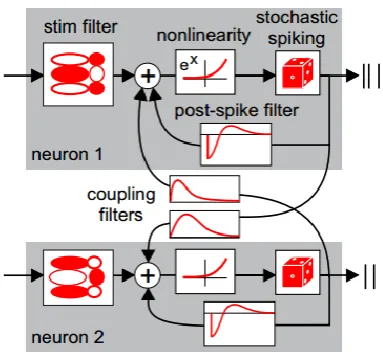
GLMs are phenomenological models that generally assume that the responses of the neurons in the current time bin are independent of each other. The response of one neuron in the current time bin may depend on the current and past stimulus and the past spiking history of the neuron itself and other neurons as shown in Figure 1.5. The probability of the response of the th
i neuron conditional on the stimulus sis given as (Truccolo et al., 2005; Pillow et al.,
2008; Latham and Roudi, 2013),
, 1
| exp ' '
i i i i i ij j
t t t t j i
q r t s K s r t h t r t t j t r t t
Z
(1.1)The first term inside the exponential takes into account the dependency of the response on the
stimulus using the stimulus filter K si
. The second term uses the post-spike filterh t
i
'
to19
histories are known. It has been used in many experimental studies investigating different cortical areas such as retina (Pillow et al., 2008), lateral geniculate nucleus (Babadi et al., 2010), motor cortex (Truccolo et al., 2010) and auditory cortex (Calabrese et al., 2011). The model with and without the dependencies on the spike trains of other neurons can be used to decode the stimuli as a way of estimating the effect of correlations (Pillow et al., 2008). GLM models were generalized to model the dependency of the neural activity on unobserved internal and external states in (Lawhern et al., 2010; Escola et al., 2011; Pfau et al., 2013). We will discuss state-spaced based analysis methods in section 1.5.5.
Figure 1.5: Illustration of the generalized linear model (GLM) for two neuron network. GLM model the response of a neuron conditional on a stimulus. The response of each neuron depends on the stimulus through the stimulus filter the dynamics of its own past spiking through the post-spike filter and the spiking dynamics of the rest of the network through coupling filters. The instantaneous firing rate is produced using a nonlinearity on the summed filter outputs. Spikes are generated using the instantaneous firing rate. (Adapted with permission from (Pillow et al., 2008))
Maximum entropy models (MEM)
20
1
| exp i i ij i j
i j i
q r t s h s r t J s r t r t
Z t
(1.2)The first term constrains the model to have the same mean firing rates for each neuron as in the data while the second term constraints the model to have the same pairwise correlations
between pairs of neurons as in the data.
Z t
is a normalization factor called partitionfunction. The model in this formulation treats the responses as stationary in time and thus does not consider the temporal dimension. However, it has been extended to include the temporal dimension by estimating the spatiotemporal probability distribution instead of the spatial distribution in (Nasser et al., 2013). Once the model is fitted, the effect of correlations could be investigated for example in an information theoretic framework using the reduction of the entropy of the probability distribution when the correlations are included in the model compared to when only the mean firing rates are included (Schneidman et al., 2006), or using mutual information between the responses and stimuli with different order of correlations included in the model (Ince et al., 2010). MEM models have been used to investigate correlations in the retina (Schneidman et al., 2006; Shlens et al., 2006; Ganmor et al., 2011; Granot-Atedgi et al., 2013; Tkacik et al., 2014), in V1 (Ohiorhenuan et al., 2010), motor cortex (Truccolo et al., 2010) and somatosensory cortex (Ince et al., 2010). As pointed out in (Roudi et al., 2009), the bin size is important for MEM models and predictions made for larger populations using models fitted to small populations or to larger time bins while assuming stationary may not always be true.
1.5.3 Decoding
21
would be one that gives reduced representations that are representative of the property being investigated and are easily interpretable in relation to the original data.
1.5.4 Mutual information
Mutual information (MI) is another generic method commonly used to study population
activity. MI
I S R
;
between a set of population response features R and the stimuli set S quantifies the reduction of uncertainty of a stimulus that can be gained from observing the response features in a single trial (Ince et al., 2010). It is calculated using the probability ofeach stimulus
P s
, the probability of observing the response features across all stimuli
P r
and the conditional probability of observing the response features for a given stimulus
|
P r s
using,
2
|
; | log
s S r R
P r s
I S R P s P r s
P r
(1.3)MI naturally accounts for all orders of interactions in the population (Ince et al., 2010). Breakdown of the full MI into subcomponents in (Pola et al., 2003) as shown below quantifies the impact of different correlative interactions in the population.
;
lin sig sim cor ind cor depI S R
I
I
I
I
(1.4)lin I
quantifies the information encoded if all cells were independent.
I
sig sim specifies how much of the information is redundant due to signal correlations that arise because the meanresponses of different neurons have similar selectivity for stimuli. Icor ind and
I
cor dep specifythe information gain or loss due to noise correlations between neurons; Icor ind is due to
correlations that do not depend on the stimulus while
I
cor dep arises because of correlationsthat depend on the stimulus.
22
combinations (for example, 7 time bins in 5 neurons) when working with a typical number of trials (~30-60 trials) (Onken et al., 2014). Therefore, it is difficult to directly generalize MI calculation to high dimensional spatiotemporal response patterns.
Some typical approaches to circumvent this problem are either to use a pooling strategy, to use an approximate probability distribution or to use a transformation or a dimensionality reduction method to reduce the dimensionality of the response space. In the first approach, all spikes of one neuron in a trial could be pooled together (i.e. pooled across time) or the responses of all neurons in one time bin could be pooled together (i.e. pooled across space) (Arabzadeh et al., 2004; Ince et al., 2013). In these cases, the population response R is
transformed to a pooled response
f R
asR
f R
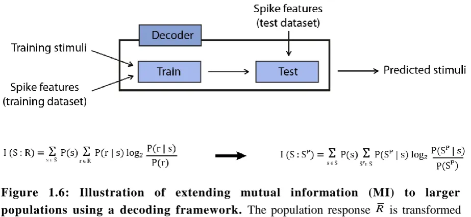
(Quian Quiroga and Panzeri, 2009). Since according to the data processing inequality, any transformation can only decrease the information in the original responses (Cover and Thomas, 2006), the MI calculated from pooling across dimensions gives a lower estimate of the information in the population. The pooling approach is only suitable if the pooled dimension has little contribution to the information encoding of the stimulus and is not suitable as a general analysis of the population activity. Under the second approach, a model such as MEM could be used as an approximate conditional probability distribution (Ince et al., 2010; Ohiorhenuan et al., 2010) or MI can be calculated under a framework of underlying Gaussian probability distributions (Yu et al., 2010; Crumiller et al., 2011). In these cases, how close the calculated MI would be to the true MI depends on how close the approximate probability distribution is to the true probability distribution. In the third approach, a decoder is trained to predict the stimulus from response features. The predicted stimulus of a decoder Sp is used as a transformation ofthe population response R as given by RSp(Quian Quiroga and Panzeri, 2009) to get a
lower estimation for MI. Alternatively, the response dimensionality can be reduced by a dimensionality reduction method such as principal component analysis (Optican and Richmond, 1987; Zuo et al., 2015). To directly relate MI values to response features, the dimensionality reduction method has to give a meaningful representation of the data.
23 1.5.5 Dimensionality reduction methods
Dimensionality reduction methods aim to describe a dataset that has a large number of data items using a few parameters (often called modules, bases, factors, hidden components or latent components) that are representative of the property being investigated (Cunningham and Byron, 2014). They are becoming increasingly important with the growth in the number of neurons that can be recorded simultaneously. Each of these methods is formulated to optimize a criterion that is specific to the method. Depending on this criterion, different methods can provide different viewpoints into a single large scale dataset. When using to analyze neural activity in space and time, dimensionality reduction methods can be broadly classified into two categories; static dimensionality reduction methods and dynamic methods (Roweis and Ghahramani, 1999; Churchland et al., 2007). Static dimensionality reduction methods first perform dimensionality reduction and subsequently formulate the time progression of the activity using the time progression of the reduced dimensional latent components. Dynamical methods on the other hand explicitly model the time progression of the neural activity, typically as the progression through a set of states.
Next we will discuss three commonly used dimensionality reduction methods; principal component analysis (PCA), independent component analysis (ICA) and factor analysis (FA) and several dynamic dimensionality reduction methods.
Static dimensionality reduction methods
Principal component analysis (PCA)
PCA extracts a set of low-dimensional components that best capture the variance in the data (Jolliffe, 2002). The components are ordered such that the first PCA component captures the highest level of variability in the dataset. The remaining components are ordered in the decreasing order of variance. All components are orthogonal to each other. A simple example of PCA applied on the spike counts recorded from two auditory cortical neurons is shown in Figure 1.7A. PCA finds that the direction that has the maximum variance in the spike counts d1 and the direction orthogonal to it d2. d1 is the low dimensional component that best
preserves the covariance between the spike counts.
24
population activity, but can confound the interpretation of the low dimensional decomposition. The low dimensional representation can also be biased by the most active neurons since the variance of spike counts increases with the mean spike count (Byron et al., 2009; Cunningham and Byron, 2014).
A variant of PCA, demixed PCA (Kobak et al., 2014) is designed to address the mixed selectivity displayed by neurons in higher cortical areas (Rigotti et al., 2013). It first marginalizes the response into independent parts that takes into account the time-varying, stimulus-dependent, decision-dependent components and their interaction. This is equivalent to the linear model used in the analysis of variance (ANOVA) test. The dimensionality reduction is performed on this marginalization with the constraint that the variance in each direction to be from only one component of the marginalization. The orthogonality constraint in PCA is relaxed in demixed PCA to allow for the demixing.
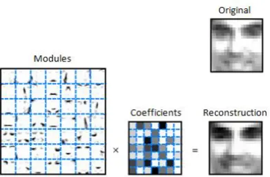
In general, identifying what the components derived from PCA represent in terms of spike counts can be difficult because they consist of both positive and negative values, whereas neural spike counts contain only non-negative values. This is more easily understood in relation to an illustration from (Lee and Seung, 1999), shown in Figure 1.7B, where PCA is applied to a dataset containing facial images. The derived module images (eigen images) contain both positive and negative values which makes it difficult to understand that they represents in terms of the visible features in the original dataset.
Figure 1.7: Principal component analysis (PCA). A: Illustration of PCA on spike counts recorded from two auditory cortical neurons. PCA finds the direction that captures the highest variance in the spike counts d1 and the direction orthogonal to it d2. B: PCA applied
to a database containing facial images extracts a set of orthonormal module images (eigen images) that best capture the variance in image pixels and a set of coefficients that indicate the contribution of each module to reconstruct an image as a linear combination of the module images. (Adapted with permission from (Lee and Seung, 1999))
Reconstructio n
Coefficients Module
25
Independent component analysis (ICA)
Independent component analysis (ICA) is used to find independent sources of activity from a mixture of activities from different sources when the sources are non-Gaussian (Comon, 1994; Hyvärinen and Oja, 2000; Brown et al., 2001). Typically, this is represented as,
s = Wx (1.5)
where the matrix s contains the independent sources to be estimated, the matrix x contains
the observed data values and Wis the demixing matrix.
Typically several preprocessing steps such as centering and whitening are performed prior to applying ICA on the data (Hyvärinen and Oja, 2000). Whitening is a linear transformation on data to derive a matrix x which contains uncorrelated components that have unit variance. Thus PCA can be used as a whitening method and ICA can be considered as an extension of PCA. Both PCA and ICA examine the dependency structure in the data. While PCA transforms data to remove the second order dependencies and decorrelates the data, ICA removes dependencies of all orders. In practice, when the sources are not strictly independent, ICA finds sources that are as independent as possible. It is based on the central limit theorem which says that the sum of a set of independent random variables will be more Gaussian than the variables themselves. ICA starts with a random vector W and rotates its axes to minimize a measure that specifies the Gaussianity such as mutual information, negentropy, kurtosis or maximum likelihood (Hyvärinen and Oja, 2000; Lopes-dos-Santos et al., 2013).
26
Factor analysis (FA)
FA assumes that the noise in the spike counts is Gaussian distributed and extracts a low-dimensional representation that models the variance in the spike counts that is shared across neurons. Simultaneously, the variance in the spike counts that is independent across neurons is identified and removed (Roweis and Ghahramani, 1999; Santhanam et al., 2009; Cunningham and Byron, 2014). Thus the method models the trial-to-trial variability in neural spike counts. More specifically, the probability distribution of the observed spike counts y of
n neurons for a given stimulus s is modeled using k Gaussian distributed independent
factors (latent components) with zero mean and unit variance x, i.e.
p
x
N
x;0, I
, such that (Santhanam et al., 2009),
,
s s,
s
p
y | x
s
N
y;μ
C x R
(1.6)and the likelihood of the spike counts for the stimulus s is,
'
,
s s s s
p y |s N y;μ C C R (1.7)
The latent variables x are considered to define the state of the population. μs is the mean number of spikes generated for the stimulus s . Cs is the nk matrix that maps the observations to the latent components. Rs is a diagonal matrix that captures the trial-to-trial variability in spike counts that is independent across neurons. This noise is attributed to the biophysical spiking noise and other non-shared sources of variability that is private to each
neuron. The covariance in y for the stimulus s is
C C
s 's
R
s.C C
s 's is the shared variabilityacross the population of neurons. This shared variability is considered to be due to the firing rate variability between neurons. FA is closely related to sensible PCA (Roweis, 1998) or probabilistic PCA (Tipping and Bishop, 1999). The difference between the two methods is that FA allows the independent noise in Rs to vary between neurons while the PCA approaches constrain it to be the same for all neurons (Santhanam et al., 2009). In general, FA works best when using bin sizes > 150 ms (Santhanam et al., 2009). Both Gaussian and Poisson noise models have been evaluated for spike count data and the Gaussian noise model achieved higher performance compared to the Poisson model (Santhanam et al., 2009).
Gaussian process factor analysis (GPFA, (Byron et al., 2009; Yu et al., 2009)) is an extension of FA that is essentially a collection of FA models applied as one FA model for each time
point in a trial. Then the neural states
x
:,tat different time points t are related through Gaussian processes. The Gaussianity gives rise to smooth trajectories of activity in time. Theth
i neural state
x
i,: is modeled as p
xi,: N
x ;0,:,t Ki
, where the T T matrix Ki defines27
2
1 2
2 2 1 21, 2 , exp 2 ,. , 2
i f i n i t t
i t t
K t t
(1.8)
The covariance of
K t t
i
1,
2 is defined from its signal variance
2f i,
, characteristic time scale i and the noise variance in the Gaussian process
n i2,
. The prior distribution ofx
:,t is set to p
x:,t N
x ;0, I:,t
and the temporal smoothness is enforced by selecting the noise variance in the Gaussian process to be small
2 3
, 10
n i
. Visualization of the model is
done after a post-processing step in which the columns of Cs are orthonomalized.
FA based models have been used to study low dimensional state trajectories in premotor and motor cortical neurons in monkeys and to model the shared firing rate variability of neurons in V1, premotor and motor cortical neurons in monkeys (Byron et al., 2009; Yu et al., 2009; Churchland et al., 2010; Afshar et al., 2011; Ecker et al., 2014; Sadtler et al., 2014).
Dynamic methods
28
Hidden Markov models (HMM)
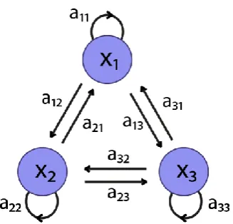
These models define one possible way in which a dynamical system could evolve across a set of unobserved (hidden) states in time, where the subsequent state that the system could take depends only on the that the system is currently in (this memorylessness defines the Markovian property). According to these models, the spiking activity of N neurons at any time instance t,yt, is in one of K discrete hidden states xt and makes a transition from one state to another according to (Escola et al., 2011),
t | [0: 1]t , [ 0:t1]
t| t 1
p x x y p x x (1.9)
Thus, the future state is dependent only on the current state and is independent of the activity in the current point in time and the history of the past states. This memorylessness is a Markovian property. Furthermore, the probability of the transition from state mto n, amn
(Figure 1.8), is constant (homogenous) at each time point with 0amn 1 and
1 1 k mn n a
.The state transition matrix A contains the elements amn . For the states to be persistent across time, the diagonal elements of A are set close to unity.
The probability of spiking, or the emission probability is modeled to be dependent only on
the current state i.e.
[ 0: 1]
[0: ]
| , |
t
t t t t
p y x y p y x . Then, if the number of spikes range between 0 to C, the probability of observing c spikes in state m, mc, mcη is given by,
|
mc
p
tc
t
y
x
m
, where 0mc 1 and1 1 C mc n
. Typically, the spike counts of each neuron are assumed to be Poisson distributed (Abeles et al., 1995; Gat et al., 1997).This gives the HMM defined by,
0 11 1
, ( ) ( | ) ( | )
T T
t t t t
t t
p p p p
y x x x x y x (1.10)
where x0 is the initial state defined by the probability distribution π such that
0
m
p
π
x
m
. The parameters of the model, A, η and π are found using maximum29
Figure 1.8: State transition diagram for a model with three hidden states. The state transition probabilities amn are specified by the state transition matrix A.
Linear dynamical models
Kalman filter and autoregressive process are two linear dynamical systems. Many of these models are based on Gaussian noise models. We will now look at each of them briefly.
Kalman filter models
The Kalman filter is a linear dynamical model describing the neural activity in terms of the observed variables (such as hand movements in a motor task) and a set of hidden states using a Gaussian noise model (Wu et al., 2009; Wu and Liu, 2015). According to this model, the neural activity yt at a time t of N neurons is related to ko number of observed variables xt
and kuo number of unobserved hidden states nt at time t by the measurement equation
t t t t
y Hx Gn v (1.11)
and the state transition is defined by the system equation
1
1
t t
t
t t
x x
A w
n n (1.12)
The Nko matrix H and the Nkuo matrix G are coefficient matrices that respectively relate the observed variables and the unobserved variables to the spike counts. A is the
k
0
k
uo
k
0
k
uo
state transition matrix similar to that for HMMs. vt and wt are30
and
p
w
t
N
0 W
,
where the NN matrix Q and the
k
0
k
uo
k
0
k
uo
matrix Wdefine the covariance of the noise. The initial state n0 is considered to be Gaussian distributed according to
p
n
0
N
μ Σ
,
such that μ is the kuo dimensional vector specifying the mean of the initial state and Σ is the kuokuo dimensional covariance matrix. The parameters of the model H G A W, , , and Q are estimated by fitting the model to thedata using maximum likelihood estimation (Wu et al., 2009). Kalman filter based models have been used to study the neural activity of motor neurons with and without the inclusion of hidden states (Wu et al., 2004; Wu et al., 2006; Wu et al., 2009).
Autoregressive models
First-order autoregressive models are typically used to model linear dynamical processes (Smith and Brown, 2003; Kulkarni and Paninski, 2007; Lawhern et al., 2010; Buesing et al., 2012a, b). The initial hidden state x0 of a model that has k states is considered to be Gaussian distributed according to
p
x
0
N
μ Σ
,
such that μ is the k dimensional vector specifying the mean of the initial state and Σ is the kk dimensional covariance matrix (Buesing et al., 2012a). The state transition is modeled by a Gaussian process
t 1|
t
t,
p
x
x
N
Ax Q
(1.13)where the kk matrix A models the temporal dependence of the process and Q is the
covariance of the state transitions. The hidden state is related to the neural activity through a
q-dimensional variable zt where zt Cxt d. C is a loading matrix that relates xt to zt
and d is the mean parameter. The neural activity is related to zt through another Gaussian process where
t|
t
t,
p
y z
N
z R
(1.14)R is the covariance of the observed neural activity at the state zt. With sufficient time
31
Summary
Advances in multi-electrode recording techniques and spike sorting methods currently allow reliable recordings from populations of hundreds of neurons simultaneously (Buzsaki, 2004; Buzsáki et al., 2015). Analyzing large ensembles is important because the brain has access to millions of neurons at the same time. Furthermore, neuroimaging methods such as fMRI allow the study of a variety of cognitive and pathological conditions noninvasively, which is often the only option when studying the human brain. However, these methods are based on large scale neuronal activity. Predicting the activity at the single cell level that gives arise to these large scale measures can only be accomplished if we understand how neurons encode information at the level of large populations.
Neurons can code information in spatial and temporal dimensions concurrently. Thus, ideally, we require methods to analyze their responses concurrently in space and time. There is a wide range of methods currently developed. However, many methods that require the evaluation of conditional probability distributions of the population responses to stimuli are constrained by the curse of dimensionality when extending to spatiotemporal analysis of large scale datasets. They often employ a range of dimensionality reduction methods to extract meaningful features from these datasets. While there is a range of dimensionality reduction methods that have been used successfully in neuroscience, it is not easy to interpret the extracted features in terms of the original data and not all methods have been used to extract information in short time scales of a few milliseconds. This indicates that there is still the need for methods that could derive representations that can give intuitively meaningful insights into understanding complex activity patterns.
1.6
Overview of the thesis
We summarized commonly used methods to study neural population coding. As we discussed, many methods are constrained by the curse of dimensionality when extending to the high dimensional spatiotemporal response space and require dimensionality reduction methods. This thesis adapts a new dimensionality reduction method, non-negative matrix factorization (NMF, (Lee and Seung, 1999)), to extract meaningful patterns of activity from the responses of large populations of neurons concurrently in space and time. NMF is a method that has been widely used in many areas within the machine learning community (Cichocki et al., 2009), but with very little application in neuroscience (Kim et al., 2005; Wei et al., 2015; Pnevmatikakis et al., 2016; Onken et al., In preparation). The thesis is organized as follows.
32
from University of Gottingen) and 3) a dataset recorded from rat barrel cortex to whisker deflections (Petersen et al., 2001). We explain in detail how our new method represents these datasets, its capability to discriminate stimuli and report findings on the spatiotemporal neural codes used by the populations.
In chapter 3, we extend space-by-time NMF to model sub-Poisson, Poisson and supra-Poisson variability in neural data, thus optimizing the model performance even further. We validate our new algorithms rigorously using statistical simulations, network simulations and applying them on our somatosensory and auditory datasets. We report the results from validation of the new update rules and detail further insight we gained in using space-by-time NMF to analyze cortical spike trains.
33
Chapter 2:
Non-negative matrix factorization to extract
spatiotemporal spike patterns
2.1
Abstract
Understanding the neural population code requires identification of salient and informative patterns of activity from large scale recordings. In this chapter we explore the feasibility of using non-negative matrix factorization (NMF) to extract informative spatiotemporal patterns of activity from recordings of spike trains from neural populations. We investigate two variations of NMF. The first, spatiotemporal NMF that identifies recurrent spatiotemporal spike patterns has been used in a few studies to study neural activity (Kim et al., 2005; Overduin et al., 2015; Wei et al., 2015). We introduce a new NMF based method space-by-time NMF (Delis et al., 2014) to study population activity.
This chapter is structured as follows. It begins with a short introduction to the importance of spatial and temporal dimensions for population coding. Next, we present a short introduction to NMF and describe the two methodologies that we use to analyze population spike trains. This is followed by a comprehensive analysis performed over three sensory datasets comprising of auditory, touch and visual modalities. We conclude the chapter with a discussion of the insight we gained through our methods and implications of using NMF to study neural activity.
2.2
Introduction
Neural populations from sensory areas (Stopfer et al., 2003; Jones et al., 2007), motor areas (Churchland et al., 2012) to higher level regions (Durstewitz et al., 2010; Mante et al., 2013) encode sensory stimuli or task-related variables using neuronal population responses with complex spatial and temporal dynamics, such as trajectories of population activity evolving across time. Understanding how these sensory, motor or task-related variables are encoded in neural population activity, that is understanding the neural population code, is a prerequisite to understand any brain function. It is important, for example, to understand what parts of neural population responses should be plotted and further analyzed in neurocognitive studies, or to understand the aspects of neural activity that must be crucially be well explained by computational models aiming at describing specific brain functions.
34
modulation of spiking activity across time (Petersen et al., 2001; Panzeri et al., 2010b; Onken et al., 2014). Spatiotemporal dynamics typically observed in populations require concurrent analysis of both dimensions. As we illustrated in section 1.5, the number of parameters that has to be estimated for a given analysis method increases exponentially when the dimensionality of the response space, as specified by the number of neurons and the duration to be analyzed, increases, but is constrained by the limited amount of trials available to estimate them (Onken et al., 2014). One common approach to overcome this curse of dimensionality is to use a dimension reduction technique (Laubach et al., 1999b; Stopfer et al., 2003; Byron et al., 2009; Churchland et al., 2012; Mazzoni et al., 2013; Zuo et al., 2015).
Dimensionality reduction methods (section 1.5.5, (Cunningham and Byron, 2014)) are mathematical procedures that describe a dataset with the smallest number of parameters and at minimal information loss. Specifically, they are designed to optimize an objective specific to each method and extract a reduced number of latent or hidden components that offer a certain viewpoint of the dataset based on the objective that the particular method optimizes. Dimension reduction methods such as principal component analysis (PCA), independent component analysis (ICA) and factor analysis (FA) have been very useful to study neural coding, the patterns they extracts from a dataset are often difficult to interpret in terms of spike counts in the original dataset. This is mainly because the patterns contain negative values which could be difficult to relate to the spike counts in the dataset.
We investigated the feasibility of using another dimension reduction method, non-negative matrix factorization (NMF), to identify salient spatial and temporal patterns from the spiking activity in large populations of neurons. NMF (Lee and Seung, 1999) is a method used in the machine learning community (Cichocki et al., 2009) to study large-scale datasets such as document and email corpuses (Xu et al., 2003; Berry and Browne, 2005) and microarray data (Brunet et al., 2004; Carmona-Saez et al., 2006). However, it is only beginning to be used to analyze neural data (Kim et al., 2005; Wei et al., 2015; Pnevmatikakis et al., 2016; Onken et al., In preparation) and limited detail is available on the low-dimensional representation with which it can represent spike data.
35
This chapter is organized as follows. It starts with a brief general introduction to NMF. Then the two methods we use to analyze data, spatiotemporal NMF and space-by-time NMF are described in detail. This is followed by findings from the three datasets using NMF to identify concurrent low-dimensional spatial and temporal patterns and its ability to discriminate stimuli in comparison to using information from only one dimension. The discussion at the end summarizes and elaborates our findings and lays out the reasons for the series of studies we conducted to improve the method to analyze neural population responses.
2.3
Non-negative matrix factorization
NMF (Lee and Seung, 1999) is a data-driven dimension reduction method that can be applied on large scale datasets containing only non-negative elements. It can extract patterns that are reliably present in the dataset at a global scale. Typically, the full dataset is arranged into a matrix. NMF can decompose this matrix into one or more matrices that contain patterns which are representative of the datasets (we refer to these matrices as module matrices) and one matrix that contains a set of weights with which each element in the original dataset could be reconstructed as a linearly weighted sum of the extracted patterns (we refer to this matrix as the coefficient matrix). The factorization process is performed iteratively where in each iteration, the factorized matrices are updated using a set of update rules designed to minimize a dissimilarity measure that quantifies the error between the original dataset and the linearly reconstructed dataset. The update rules are constrained such that the factorized matrices remain non-negative throughout the updating process. This non-negativity constraint together with the linear reconstruction give rise to identification of patterns that are sparse and part-based (Lee and Seung, 1999). They are often found to have clear and intuitive meaning with respect to the original data in many areas that have used NMF as a dimension reduction method. A few representative data types include facial images (Lee and Seung, 1999; Guillamet and Vitria, 2002), document and email corpuses (Xu et al., 2003; Berry and Browne, 2005), microarray data (Brunet et al., 2004; Carmona-Saez et al., 2006), electromyographic activity (d'Avella et al., 2003; Delis et al., 2013; Delis et al., 2014) and music (Smaragdis and Brown, 2003; Févotte et al., 2009).
NMF in its basic two-factor decomposition (Lee and Seung, 1999) factorizes a NT matrix
R into a NK module matrix W and a K T coefficient matrix H where,
R WH (2.1)
and
K
min
T N
,
. The module matrix W consists of the low-dimensional patterns36
In the example shown in Figure 2.1, NMF was applied on a facial image dataset (Lee and Seung, 1999). The data matrix R was constructed such that each column in R contained the intensity of the vectorized pixels in one image. Each module extracted into W matrix is an image consisting of a global facial feature in the dataset such as eyes, nose or lips. The coefficients in the H matrix indicate the level of the presence of each facial feature within each image. The reconstruction of an image in the dataset ri is obtained as
1
K