R E S E A R C H
Open Access
An augmented Lagrangian method for the
Signorini boundary value problem with BEM
Shougui Zhang
*and Xiaolin Li
*Correspondence: [email protected] School of Mathematical Sciences, Chongqing Normal University, Chongqing, 401331, P.R. China
Abstract
We analyze augmented Lagrangian and boundary element methods for the Signorini boundary value problem of Laplacian. The boundary variational formulation is presented by the boundary integral operators, and the Signorini boundary conditions are formulated as a fixed point problem. Semismooth Newton methods are applied for the numerical solution of the problem. We prove the convergence of the method and confirm the theory by some numerical experiments.
Keywords: Signorini boundary conditions; fixed point; augmented Lagrangian; boundary element; semismooth Newton methods
1 Introduction
Signorini boundary value problems are of great importance in many applications, such as the electropaint process and contact problem [–],etc.These problems involve inequality constraints on a part of the boundary that make them nonlinear. Therefore, development of efficient numerical algorithms for Signorini boundary value problems is one of the most important branches of modern computational mathematics and mechanics. Usually Sig-norini boundary value problems have been considered mathematically and numerically with variational inequalities, especially by the finite element method (FEM) [–] and the boundary element method (BEM) [–]. Recently, sound and efficient algorithms for the solution of these problems were still a very active field of research (see [–]).
As we know, the fixed point method based on projection theory is a powerful tool to deal with complementary problems and variational inequalities in finite dimensional space []. The main idea of this method is to establish the equivalence between the original problem and the fixed point problem by using projection. This equivalent formulation plays a significant role in developing various iterative methods for solving an original prob-lem. During the last years, a number of projection methods have been studied exten-sively [, , , ], which are perfectly efficient for solving the problem. In these meth-ods, the problem has been formulated by a projection algorithm, and no other inequality constraint is needed. Consequently, the method is easy to implement for the numerical solution and the proof of convergence is very simple.
In the case of Signorini boundary conditions, the unknown boundary values are the potential and its derivative on the boundary, which are considered primary variables in BEM. They can be obtained directly using boundary integral equations [, ]. There-fore, the method combining the projection method with the BEM is more appropriate for
Signorini boundary value problems [–]. However, few investigations have been done on the Signorini boundary value problem by the augmented Lagrangian and fixed point methods with the BEM.
In this paper, we focus on the boundary augmented Lagrangian methods (BALM) for the solution of Signorini boundary value problems, which is inspired by classical augmented Lagrangian methods (ALM) [] and the BEM []. First of all, we deduce the boundary weak formulation with Steklov-Poincaré operator. Second, we use the projection tech-nique to deal with the Signorini boundary conditions by an equality and the projection. Although the new problem is still nonlinear on the boundary, this problem no longer has the inequality constraint and can be solved by the semismooth Newton method with local superlinear convergence rate [, ]. Using these transformations, we propose a BALM for the Signorini boundary value problem, which only needs the iteration for boundary func-tion and the computafunc-tion of the boundary variafunc-tional equafunc-tion. Then we can use proper-ties of the projection and the boundary integral operator to prove the convergence of the method. Numerical results show that our method is accurate and efficient.
The structure of the paper is as follows. In Section , we first describe the classical Signorini boundary value problem and use the Steklov-Poincaré operator to introduce the variational formulation. Then we establish equivalent formulations between the non-linear boundary conditions and the fixed point problem, and propose a new ALM for the problem. Section is devoted to the convergence analysis of the method, which shows monotone convergence properties of the numerical solution toward the solution of the original problem. In Section , we present some numerical experiments to investigate the performance of our method, and finally a brief conclusion is given in Section .
2 The weak formulations for the Signorini boundary-value problem
Let⊂Rbe a bounded domain with a Lipschitz boundaryand outward unit normaln. This boundary consists of three disjoint parts, the Dirichlet boundaryD, the Neumann boundaryNand the Signorini boundaryS=∅. For simplicity, we consider the Signorini boundary value problem for the Laplace equation: findu∈H() such that
u= in, (.)
u=g onD, (.)
λ=f onN, (.)
u≥g, λ≥f, (u–g)(λ–f) = onS, (.)
whereλ:=∂u
∂n,g∈H
/(\ ¯
N), andf ∈H–/(\ ¯D) are given. We note thatH–/(\ ¯D) is defined by the dual ofH/(\ ¯D) :={u∈H/(\ ¯D)|suppu⊂ ¯}with the norm
fH–/(\ ¯
D):= sup
=v∈H/(\ ¯
D)
|f,v\ ¯D| vH/(\ ¯
D) .
Here·,·\ ¯D denotes the extension of the usualL
(\ ¯
D) scalar product toH–/(\
¯
D)×H/(\ ¯D). It is well known in the theory of variational inequalities that this prob-lem has a unique solution ifS=∅or
We define the space of functions as
HD() :=v∈H(),v=gonD
.
Applying the Green’s formula, we obtain the variational formulation from (.)-(.) as follows:
∇u∇v dx=
N∪S
λv ds, ∀v∈HD(). (.)
Further, we introduce the Dirichlet-to-Neumann map on[, , ]
S: H/()→H–/()
u|→λ|.
InsertingS(u|) =λ|into (.) yields
∇u∇v dx=
S(u|)v ds, ∀v∈HD(),
where the Steklov-Poincaré operatorSis defined by
(Su)(x) =
D+
I+K
V–
I+K u(x) (.)
with the boundary integral operators
(Vλ)(x) =
U(x,y)λ(y)dsy, V:H–/()→H/(),
(Ku)(x) =
∂ ∂ny
U(x,y)u(y)dsy, K:H/()→H/(),
Kλ(x) =
∂ ∂nx
U(x,y)λ(y)dsy, K:H–/()→H–/(),
(Du)(x) = – ∂
∂nx
∂ ∂ny
U(x,y)u(y)dsy, D:H/()→H–/().
Here the functionUis the fundamental solution of the two-dimensional Laplace equation:
U(x,y) = –
πln|x–y|.
Let us define
HD/() :=v∈H/(),v=gonD
,
H/(,D) :=
v∈H/(),v= onD
,
Su,v:=
Su(x)v(x)dsx,
λ,vS:=
S
L(v) :=
N
f(x)v(x)dsx.
We then can obtain the boundary weak formulation of the problem (.)-(.) as fol-lows:
Su,v–λ,vS=L(v), ∀v∈H
/
D (). (.)
It can be proved that the Steklov-Poincaré operator Sis bounded and symmetric, and semielliptic onH/(). We will use the following property for the operatorS[].
Lemma . The Steklov-Poincaré operator S defined by(.)is elliptic on H/(,D),
Sv,vL()≥αv
H/(), (.)
whereαis a positive constant.
On the other hand, we can transfer the nonlinear boundary conditions (.) to a fixed point problem [, , , , , ]. Let us introduce the projection notation forv∈R:
[v]+=
v ifv> , otherwise.
Consequently, we obtain the following result [, ].
Lemma . For allρ> ,the boundary conditions(.)onSare equivalent to:
u–g–u–g–ρ(λ–f)+= onS. (.)
Proof Letube such that (.) holds. Considering the conditionu≥gwe have eitheru>g
oru=g. First, suppose thatu>g. Then the condition (u–g)(λ–f) = implies thatλ=f. Therefore, we have
u–g–ρ(λ–f)+= [u–g]+=u–g.
Then suppose thatu=g. The conditionλ≥f can also be rewritten as [–ρ(λ–f)]+= , so
it follows that
u–g–ρ(λ–f)+=–ρ(λ–f)+= =u–g.
On the other hand, letuandλbe such that (.) holds. Note first that it impliesu≥g. Consider first the caseu=g. Equation (.) can be rewritten as [–ρ(λ–f)]+= , which is
equivalent to the condition
λ≥f.
Sinceu=g, the following condition also holds:
We now consider the caseu>g. From (.), [u–g–ρ(λ–f)]+> , so that in this case
u–g= [u–g–ρ(λ–f)]+=u–g–ρ(λ–f), from which we have
λ=f,
so that all conditions in (.) hold.
Now, we obtain the boundary weak formulation (.) by the Steklov-Poincaré operatorS
and the fixed point problem (.) for the problem (.)-(.), which only involves a bound-ary integral operator and no inequality constraint. This alternative equivalent formulation is also useful from the numerical and theoretical analysis point of view. With the above preparations, we can now list our boundary augmented Lagrangian method (BALM) for the Signorini boundary value problem as below.
Algorithm BALM
Step : Chooseu()∈L(
S),ρ∈R+, and setk:= .
Step : Solve
Su(k+),v+λ(k+),v
S=L(v), ∀v∈H
/
D (), (.)
with boundary condition
u(k+)–g–u(k)–g–ρλ(k+)–f+= onS, (.)
and obtainu(k+)andλ(k+)onS.
Step : Update (.) byk:=k+ and return to Step .
For the nonlinear problem (.), we can apply the semismooth Newton method for its solution [, ]. In the next section the convergence of the algorithm is analyzed.
3 Convergence of the algorithm
Letu∗ andλ∗ denote the solution of Signorini boundary value problem and the corre-sponding derivative on the boundary, respectively. In order to analyze the convergence of the method in Section , we suppose that the sequencesu(k)∈H/() andλ(k)∈L(
S). Now, we define
Bρ(u,λ) :=u–g–ρ(λ–f),
and we have the following projection property onS[, , ].
Lemma . For all u(k)∈H/()andλ(k)∈L(
S)generated by the BALM,
u(k+)–u∗,Bρu(k),λ(k+)–Bρu∗,λ∗ S≥u
(k+)–u∗
S. (.)
Proof We separateSinto the four subpartsS,S,S, andS, where
Bρu(k),λ(k+)≥,Bρu∗,λ∗< onS,
Bρu(k),λ(k+)< ,Bρu∗,λ∗≥ onS,
Bρu(k),λ(k+)< ,Bρu∗,λ∗< onS.
Using (.) and (.) we then get
u(k+)–u∗=Bρu(k),λ(k+)–Bρu∗,λ∗ onS,
≤u(k+)–u∗=Bρu(k),λ(k+)– <Bρu(k),λ(k+)–Bρu∗,λ∗ onS,
≥u(k+)–u∗= –Bρu∗,λ∗>Bρu(k),λ(k+)–Bρu∗,λ∗ onS,
u(k+)–u∗= – = onS.
Consequently,
u(k+)–u∗,Bρu(k),λ(k+)–Bρu∗,λ∗ S≥u
(k+)–u∗
S.
Theorem . Let{(u(k),λ(k))}be the sequence generated by the BALM,for all k then u(k) converges to u∗in H/()andλ(k)converges toλ∗in L(S)as k→ ∞.
Proof Noteδu(k):=u(k)–u∗∈H/(,D) andδ(λk):=λ(k)–λ∗∈L(S). Considering that (u∗,λ∗) satisfies (.) we obtain
Su∗,δu(k+)–λ∗,δ(uk+) S=L
δ(uk+). (.)
From (.) of BALM we have
Su(k+),δu(k+)–λ(k+),δ(uk+) S=L
δ(uk+). (.)
Subtracting (.) from (.) yields
Sδu(k+),δu(k+)=δλ(k+),δ(uk+)
S. (.)
Using Lemma . and Young’s inequality
δλ(k),δu(k+) S≤
δ
(k)
λ
S+δ
(k+)
u S , we obtain
δλ(k+),δ(uk+) S =ρ
–δ(k)
u ,δu(k+)
S–ρ
–Bρu(k),λ(k+)–Bρu∗,λ∗,δ(k+)
u
S
≤ρ–δu(k),δu(k+) S–ρ
–δ(k+)
u
S
≤(ρ)–δu(k) S– (ρ)
–δ(k+)
u
S.
From (.) and Lemma . we then have
Sδu(k+),δu(k+)≤(ρ)–δu(k) S– (ρ)
–δ(k+)
u
and
Sδu(k+),δu(k+)≥αδ(uk+)
H/(). (.)
It follows from (.) and (.) that
αδu(k+)H/()≤(ρ)–δu(k)
S– (ρ)
–δ(k+)
u
S. (.)
Then
∞
k=
αδu(k+)H/()≤(ρ)–δu()
S<∞.
Consequently,
lim
k→∞δ
(k+)
u
H/()= .
Thusu(k)converges tou∗inH/() and from (.) of BALMλ(k)converges toλ∗inL(
S)
ask→ ∞.
According to (.), the sequence{u(k)}is bounded and the sequence{δ(k)
u S}is mono-tonically decreasing. Furthermore, we can see that the larger value of the parameterρ
results in faster convergence to the algorithm.
4 Numerical experiments
To test the numerical verification of the theory, the algorithm above has been implemented and applied to some examples of Signorini problems in this section. An analytic solution is known for the first example, and the exact solution for the two other examples is not known. For the sake of simplicity, we apply a constant BEM to the problem (.) with iterations. Here, we chooseu(k+)–u(k)
∞,S≤–u(k+)∞,S as a stopping criterion. 4.1 Dirichlet-Signorini problem
First we consider a Signorini boundary value problem in an annular domain={(x,y) :
a<x+y <b} with a Dirichlet boundary condition on the boundary
D ={(x,y) :
x+y =b} ∪ {(x,y) :x+y=a,y≥} and a Signorini boundary condition on the
S=\ ¯D. The analytic solution in the domain is given by the following complex function:
u(x,y) =Imω(x+iy), where
ω(x+iy) =
x–y
r + r
a –
a
r
+
x–y
r
r
a +
a r signx +i
x–y
r + r
a–
a
r
–
x–y
r
r
a+
a
r
andr=x+y,x+y≥a. For this problem, we can easily obtain the Dirichlet
bound-ary condition onDfrom the analytic solution, and the Signorini boundary condition is given by
u≥, λ≥, uλ= onS.
The analytic solution of this problem and its normal derivative on the Signorini boundary
Sare
u(x,y) =
max
,x
–y
a
signy, (.)
λ(x,y) = –
a
max
,x
–y
a
|x|y. (.)
Using the BEM, this problem has been considered by the decomposition-coordination method [], the projection iterative algorithm [], and the linear complementary method [],etc.
We consider the casesa= . andb= . and introduce the parameterizationst→
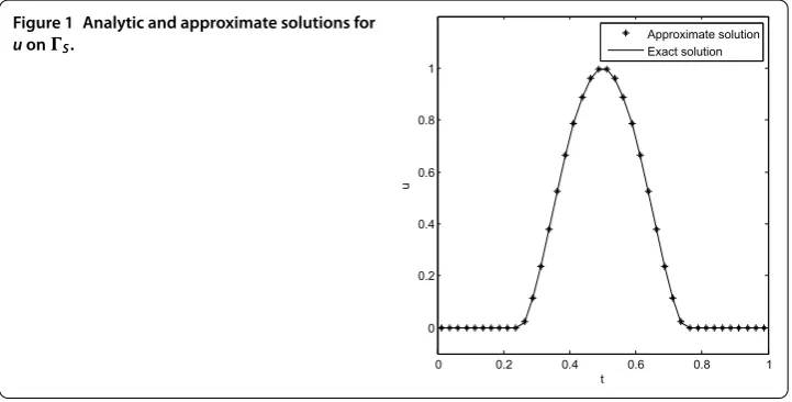
(acosπt, –asinπt) andt→(bcosπt,bsinπt). First we chooseρ= , and apply our method to this problem on a uniform grid fort. The discretization includes boundary elements onSand boundary elements onD, soN= . Figure plots the approxi-mations and exact solutions for the potentialuonS. The results for the normal derivative
λare shown in Figure . These figures show that our results are in excellent agreement with the exact solution (.) and (.).
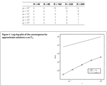
To verify the convergence of our method, we solve the problem by choosing dif-ferent numbers of boundary elements N and various values of the parameter ρ. Ta-ble shows the number of iterations with N = , , , , and on andρ= , , , , , and . We can observe that the numerical results show good
con-vergence as the parameter ρ increases. Moreover, the number of iterations increases
Figure 1 Analytic and approximate solutions for
Figure 2 Analytic and approximate solutions for λonS.
Table 1 Number of iterations with different values ofNandρ
N = 40 N = 80 N = 160 N = 320 N = 640
ρ= 100 9 9 10 10 12
ρ= 101 6 6 7 8 8
ρ= 102 5 5 6 7 8
ρ= 103 4 4 5 6 7 ρ= 104 3 4 5 6 7 ρ= 105 3 4 5 6 7
Figure 3 Log-log plot of the convergence for approximate solutionsuonS.
slowly asNincreases. We define the error
e(u) =
NS NS
i=
u(xi) –uh(xi),
whereNSdenotes the number of boundary elements onS, andu(xi) anduh(xi) denote exact and numerical solutions, respectively. Here we draw the error with the logarithmic scale depending on the steph. Figures and display the change trend of the error foru
Figure 4 Log-log plot of the convergence for approximate solutionsλonS.
4.2 Dirichlet-Signorini problem
Second, we consider the following Signorini boundary value problem known as the steady-state electropainting problem:
u= in= (–., .)×(, ),
u= onD=
(x,y) : –.≤x≤.,y= ,
with the following Signorini boundary conditions
u≥, λ≥–ε, u(λ+ε) = onS,
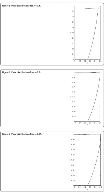
whereS=\ ¯D. This problem has been extensively considered by different methods [, , , ].
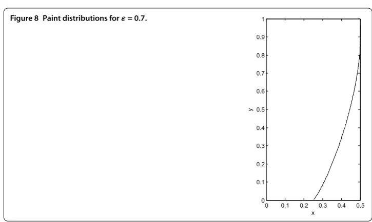
In this problem the Signorini boundary conditions describe the location of these painted and unpainted parts onS, and the solution of the problem depends on the value ofε. We now apply our method to this problem, and four cases with different values ofεare considered. Here, we chooseN= andρ= again, and we let uε denote the paint thickness. We only consider the paint distribution over half the boundary because the problem is symmetric, and the numerical results corresponding toε= .,ε= .,ε= ., andε= . are presented in Figures -, respectively. It can be observed that our results are in good agreement with the corresponding results in [, , ].
We also investigate the convergence behavior of our method for this example. Tables - display the number of iterations for the four cases with differentNandρ. As can be seen from our tests, our method converges quickly whenρis sufficiently large and the number of iterations depends only weakly onN.
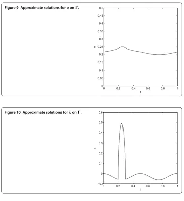
4.3 Signorini problem
Finally, we consider a Signorini boundary value problem in a domain defined by an el-lipse [],
Figure 5 Paint distributions forε= 0.4.
Figure 6 Paint distributions forε= 0.5.
Figure 8 Paint distributions forε= 0.7.
Table 2 Number of iterations forε= 0.4 with differentNandρ
N = 40 N = 80 N = 160 N = 320 N = 640
ρ= 100 48 48 47 47 46 ρ= 101 15 15 16 16 16 ρ= 102 9 9 10 11 11
ρ= 103 8 8 9 9 9
ρ= 104 7 7 8 9 9
ρ= 105 6 6 7 8 8
Table 3 Number of iterations forε= 0.5 with differentNandρ
N = 40 N = 80 N = 160 N = 320 N = 640
ρ= 100 22 25 24 25 24
ρ= 101 11 11 12 13 13
ρ= 102 8 9 9 11 11
ρ= 103 7 8 9 10 10 ρ= 104 6 7 8 10 10 ρ= 105 6 7 8 9 9
Table 4 Number of iterations forε= 0.55 with differentNandρ
N = 40 N = 80 N = 160 N = 320 N = 640
ρ= 100 22 20 21 21 21 ρ= 101 10 11 11 12 12 ρ= 102 8 8 9 10 10 ρ= 103 7 7 8 9 10 ρ= 104 6 6 8 9 10 ρ= 105 6 6 8 9 9
Table 5 Number of iterations forε= 0.7 with differentNandρ
N = 40 N = 80 N = 160 N = 320 N = 640
Figure 9 Approximate solutions foruon.
Figure 10 Approximate solutions forλon.
Table 6 Number of iterations with differentNandρ
N = 40 N = 80 N = 160 N = 320 N = 640
ρ= 100 43 46 46 45 46 ρ= 101 15 16 17 17 18 ρ= 102 10 11 13 13 14 ρ= 103 8 10 12 12 13 ρ= 104 8 9 11 11 13 ρ= 105 7 9 11 11 13
with the Signorini boundary conditions
u≥x+y, λ≥–x, u–x–yλ+x= on=∂E(a,b),
that the algorithm also converges quickly and the numbers of iterations decrease as ρ
increases, and a differentNhas little effect on the numbers of iterations.
5 Conclusion
In this paper, we have proposed a new ALM for the solution of Signorini boundary value problems and proven its convergence. Using the BEM and the fixed point method, we can easily apply this algorithm to the Signorini boundary value problems defined in domains of arbitrary shape. Each iteration only needs to solve an elliptic variational problem and the semismooth Newton method is used to find the solution. The examples tested show the feasibility and effectiveness of the algorithm.
Competing interests
The authors declare that they have no competing interests.
Authors’ contributions
All authors equally have made contributions. All authors read and approved the final manuscript.
Acknowledgements
This work was funded by China Scholarship Council, the Natural Science Foundation Project of CQ CSTC of China (Grant Nos. cstc2013jcyjA30001 and cstc2013jcyjA10049) and Fundamental Research Funds of Chongqing Normal University of China (Grant No. 13XLB001), the National Natural Science Foundation of China (Grant Nos. 11471063 and 11301575).
Received: 9 October 2015 Accepted: 5 March 2016 References
1. Glowinski, R: Numerical Methods for Nonlinear Variational Problems. Springer, Berlin (2008)
2. Aitchison, JM, Lacey, AA, Shillor, M: A model for an electropaint process. IMA J. Appl. Math.33, 269-287 (1984) 3. Chouly, F, Hild, P: A Nitsche-based method for unilateral contact problems: numerical analysis. SIAM J. Numer. Anal.
51, 1295-1307 (2013)
4. Ryoo, CS: Numerical verification of solutions for Signorini problems using Newton-like method. Int. J. Numer. Methods Eng.73, 1181-1196 (2008)
5. Ryoo, CS: An approach to the numerical verification of solutions for variational inequalities using Schauder fixed point theory. Bound. Value Probl.2014, Article ID 235 (2014)
6. Hild, P, Renard, Y: An improveda priorierror analysis for finite element approximations of Signorini’s problem. SIAM J. Numer. Anal.50, 2400-2419 (2012)
7. Stadler, G: Path-following and augmented Lagrangian methods for contact problems in linear elasticity. J. Comput. Appl. Math.203, 533-547 (2007)
8. Han, HD: A direct boundary element method for Signorini problems. Math. Comput.55, 115-128 (1990) 9. Spann, P: On the boundary element method for the Signorini problem of the Laplacian. Numer. Math.65, 337-356
(1993)
10. Steinbach, O: Boundary element methods for variational inequalities. Numer. Math.126, 173-197 (2014)
11. Maischak, M, Stephan, EP: Adaptivehp-versions of BEM for Signorini problems. Appl. Numer. Math.54, 425-449 (2005) 12. Mel’nyk, TM: Homogenization of the Signorini boundary-value problem in a thick junction and boundary integral
equations for the homogenized problem. Math. Methods Appl. Sci.34, 758-775 (2011)
13. Aitchison, JM, Poole, MW: A numerical algorithm for the solution of Signorini problems. J. Comput. Appl. Math.94, 55-67 (1998)
14. Ito, K, Kunisch, K: Semi-smooth Newton methods for the Signorini problem. Appl. Math.53, 455-468 (2008) 15. Bustinza, R, Sayas, FJ: Error estimates for an LDG method applied to Signorini type problems. J. Sci. Comput.52,
322-339 (2012)
16. Karageorghis, A, Lesnic, D, Marin, L: The method of fundamental solutions for solving direct and inverse Signorini problems. Comput. Struct.151, 11-19 (2015)
17. Wang, F, Han, WM, Cheng, XL: Discontinuous Galerkin methods for solving the Signorini problem. IMA J. Numer. Anal.
31, 1754-1772 (2011)
18. Li, F, Li, XL: The interpolating boundary element-free method for unilateral problems arising in variational inequalities. Math. Probl. Eng.2014, Article ID 518727 (2014)
19. Zhang, SG, Zhu, JL: A projection iterative algorithm boundary element method for the Signorini problem. Eng. Anal. Bound. Elem.37, 176-181 (2013)
20. Zhang, SG: A projection iterative algorithm for the Signorini problem using the boundary element method. Eng. Anal. Bound. Elem.50, 313-319 (2015)
21. Cottle, RW, Pang, JS, Stone, RE: The Linear Complementarity Problem. Academic Press, Boston (1992) 22. He, BS, Liao, LZ: Improvements of some projection methods for monotone nonlinear variational inequalities.
J. Optim. Theory Appl.11, 111-128 (2002)
23. Noor, MA: Some developments in general variational inequalities. Appl. Math. Comput.152, 199-277 (2004) 24. Hsiao, GC: Boundary Integral Equations. Springer, Berlin (2008)