The Thirty-Third AAAI Conference on Artificial Intelligence (AAAI-19)
Attentive Tensor Product Learning
Qiuyuan Huang
Microsoft Research Redmond, WA, USA [email protected]
Li Deng
Citadel, USA [email protected]
Dapeng Wu
University of Florida Gainesville, FL, USA
Chang Liu
Citadel Securities Chicago, IL, USA [email protected]
Xiaodong He
JD AI Research Beijing, China [email protected]
Abstract
This paper proposes a novel neural architecture — Attentive Tensor Product Learning (ATPL) — to represent grammatical structures of natural language in deep learning models. ATPL exploits Tensor Product Representations (TPR), a structured neural-symbolic model developed in cognitive science, to in-tegrate deep learning with explicit natural language structures and rules. The key ideas of ATPL are: 1) unsupervised learn-ing of role-unbindlearn-ing vectors of words via the TPR-based deep neural network; 2) the use of attention modules to com-pute TPR; and 3) the integration of TPR with typical deep learning architectures including long short-term memory and feedforward neural networks. The novelty of our approach lies in its ability to extract the grammatical structure of a sen-tence by using role-unbinding vectors, which are obtained in an unsupervised manner. Our ATPL approach is applied to 1) image captioning, 2) part of speech (POS) tagging, and 3) constituency parsing of a natural language sentence. The experimental results demonstrate the effectiveness of the pro-posed approach in all these three natural language processing tasks.
1
Introduction
Deep learning is an important tool in many speech and natu-ral language processing (NLP) applications (Hinton and oth-ers 2012; Deng and Liu 2018). Since natural language is rich in grammatical structures, there has been an increasing inter-est in learning a vector representation to capture the gram-matical structures of the natural language descriptions using deep learning models in recent years (Tai, Socher, and Man-ning 2015; Kumar et al. 2016; Kong et al. 2017).
In this work, we propose a new architecture, called Atten-tive Tensor Product Learning (ATPL), to address this repre-sentation problem by exploiting Tensor Product Represen-tations (TPR) (Smolensky and Legendre 2006; Smolensky et al. 2016; Palangi et al. 2017; Huang et al. 2017). TPR is a structured neural-symbolic model developed in cogni-tive science over 20 years ago. In the TPR theory, a sen-tence can be considered as a sequence ofroles(i.e., gram-matical components) where each role is connected to afiller
(i.e., tokens). Given each role associated with arole vector
Copyright c2019, Association for the Advancement of Artificial Intelligence (www.aaai.org). All rights reserved.
rtand each filler associated with afiller vectorft, the TPR
of a sentence can be computed asS =P tftr
>
t . Comparing
with the popular RNN-based representations of a sentence, a good property of TPR is that decoding a token of a time stamptcan be computed directly by providing anunbinding vectorut. That is,ft =S·ut. Under the TPR theory,
en-coding and deen-coding a sentence is equivalent to learning the role vectorsrtor unbinding vectorsutat each positiont.
We employ the TPR theory to develop a novel attention-based neural network architecture for learning the unbinding vectors ut that serve as the core of ATPL. That is, ATPL
employs a form of recurrent neural networks to produceut
one at a time. In each time, the TPR of the partial prefix of the sentence up to timet−1 is leveraged to compute the attention maps, which are then used to compute the TPR
St as well as the unbinding vector ut at time t. In doing
so, our ATPL can not only be used to generate a sequence of tokens, but also be used to generate a sequence ofroles, which can in turn interpret the syntactic/semantic structures of the sentence.
To demonstrate the effectiveness of our ATPL architec-ture, we apply it to three important NLP tasks: 1) image captioning; 2) POS tagging; and 3) constituency parsing of a sentence. The first task showcases our ATPL-based gen-erator, while the latter two tasks are used to demonstrate the power of role vectors in interpreting sentences’ syntac-tic structures. Our evaluation shows that on both image cap-tioning and POS tagging, our approach can outperform pre-vious state-of-the-art approaches. In particular, on the con-stituency parsing task, when the structural segmentation is given as a ground truth, our ATPL approach can beat the state-of-the-art by3.5to4.4points on the Penn TreeBank dataset. These results demonstrate that our ATPL is highly effective in capturing the syntactic structures of natural lan-guage sentences.
2
Related Work
Our proposed method for image captioning, the first NLP task we consider in this paper, follows a great deal of recent caption-generation literature on exploiting end-to-end deep learning with a CNN image-analysis front end producing a distributed representation that is then used to drive a natural-language generation process, typically using RNNs (Mao et al. 2015; Vinyals et al. 2015b; Karpathy and Fei-Fei 2015). Our grammatical interpretation of the structural roles of words in sentences is connected with other work that also in-corporates deep learning into grammatically-structured net-works (Tai, Socher, and Manning 2015; Andreas et al. 2015; Yogatama et al. 2016; Maillard, Clark, and Yogatama 2017). In these earlier studies, the network itself is not structured to match the grammatical structure of sentences being pro-cessed. In our work, the structure is fixed, but it is designed to support the learning of distributed representations that incorporate structure internal to the representations them-selves — filler/role structure.
The second NLP task we consider in this paper is POS tagging. Methods for automatic POS tagging are our base-lines. They include unigram tagging, bigram tagging, tag-ging using Hidden Markov Models (which are generative se-quence models), maximum entropy Markov models (which are discriminative sequence models), rule-based tagging, and tagging using bidirectional maximum entropy Markov models (Jurafsky and Martin 2017). The celebrated Stanford POS tagger of (Manning 2017) uses a bidirectional version of the maximum entropy Markov model called a cyclic de-pendency network in (Toutanova et al. 2003).
Methods for automatic constituency parsing, the third NLP task tackled in this paper, include those based on probabilistic context-free grammars (CFGs) (Jurafsky and Martin 2017), the shift-reduce method (Zhu et al. 2013), sequence-to-sequence LSTMs (Vinyals et al. 2015a). Our constituency parser is similar to the sequence-to-sequence LSTMs (Vinyals et al. 2015a) since both use LSTM neu-ral networks to design a constituency parser. Different from (Vinyals et al. 2015a), our constituency parser uses TPR and unbinding role vectors to extract features that contain gram-matical information.
3
Attentive Tensor Product Learning
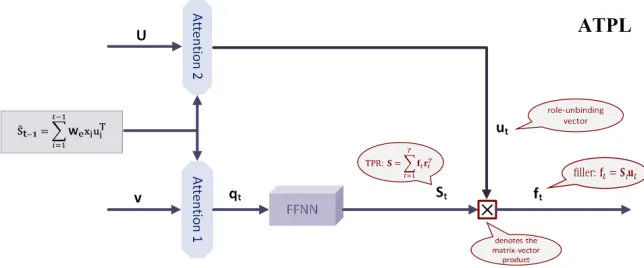
In this section, we present the ATPL architecture. We will first briefly revisit the Tensor Product Representation (TPR) theory, and then introduce several building blocks. In the end, we explain the ATPL architecture, which is illustrated in Figure 1.
3.1
Background: Tensor Product Representation
The TPR theory allows computing a vector representation of a sentence as the summation of its individual tokens while the order of the tokens is represented implicitly (Smolensky 1990; Huang et al. 2018; Lee et al. 2016). For a sentence ofT words, denoted byx1,· · ·, xT, TPR theory considers
the sentence as a sequence ofgrammatical role slotswith each slot filled with a concrete token xt. The role slot is
often shortened and referred to as arole, while the tokenxt
referred to as afiller.
The TPR of the sentence can thus be computed asbinding
each role with a filler. Mathematically, each role is associ-ated with a role vector rt ∈ Rd, and a filler with a filler
vectorft∈Rd. Then the TPR of the sentence is
S= T X
t=1
ft·r>t (1)
whereS ∈ Rd×d. Each role is also associated with a dual
unbinding vectorutso thatrt>ut= 1andr>tut0 = 0, t0 6=t;
then
ft=Sut (2)
Intuitively, Eq. (2) requires that R>U = I, where R = [r1;· · · ;rT],U = [u1;· · · ;uT], and Iis an identity
ma-trix. In a simplified case, i.e.,rtis orthogonal to each other
andrt>rt= 1, we can easily deriveut=rt.
Eqs. (1) and (2) provide means tobindingorunbindinga TPR. Through these mechanisms, one can easily construct an encoder and a decoder to convert between a sentence and its TPR. All we need to compute is the role vectorrt(or its
dual unbinding vectorut) at each time stept.
3.2
Building blocks
Before we start introducing ATPL, we first introduce several building blocks repeatedly used in our construction.
Anattention moduleover an input vectorvis defined as
Attn(v) =σ(W v+b) (3)
whereσis the sigmoid function,W ∈Rd1×d2,b∈
Rd1,d2 is the dimension of v, andd1 is the dimension of the out-put. Intuitively,Attn(·)will output a vector as the attention heatmap, andd1is its dimension.W andbare two sets of parameters. Without specific notices, the sets of parameters of different attention modules are disjoint to each other.
We refer to a Feed-Forward Neural Network (FFNN) module as a single fully-connected layer:
FFNN(v) =tanh(W v+b) (4)
whereW andbare the parameter matrix and the parameter vector with appropriate dimensions respectively, andtanh
is the hyperbolic tangent function.
3.3
ATPL architecture
In this paper, we mainly focus on an ATPL decoder archi-tecture that can decode a vector representationvinto a se-quencef1,· · ·, fT. The architecture is illustrated in Fig. 1.
If we require that the role vectors be orthogonal to each other, then to decode the fillerftonly needs to unbind the
TPR of undecoded words,St:
ft=Stut= T X
i=t
(Wexi)ri>
ut=Wext (5)
wherext ∈RV is a one-hot encoding vector of dimension
Figure 1: ATPL Architecture.
embedding matrix, thei-th column of which is the embed-ding vector of thei-th word in the vocabulary. We can use any algorithm to obtain the word embedding vectors; in this work, we choose the Stanford GLoVe algorithm with zero mean (Pennington, Socher, and Manning 2017).
To computeStandut, ATPL employs two attention
mod-ules controlled byS˜t−1, which is the TPR of the so-far
gen-erated wordsx1,· · · , xt−1:
˜
St−1=
t−1
X
i=1
Wexir>i
On one hand,Stis computed as follows:
qt = vAttn(ht−1⊕vec( ˜St−1)) (6)
St = FFNN(qt) (7)
where is the point-wise multiplication, ⊕concatenates two vectors, andvec vectorizes a matrix. In this construc-tion,ht−1is the hidden state of an external LSTM, which we will explain later.
The key idea here is that we employ an attention model to place weights on each dimension of the vectorv, so that it can be used to computeSt. Note it has been demonstrated
that attention structures can be used to effectively learn any function (Vaswani et al. 2017). Our work adopts a similar idea to computeStfromvandS˜t−1.
On the other hand, similarly,utis computed as follows:
ut=UAttn(ht−1⊕vec( ˜St−1))
whereUis a constant normalized Hadamard matrix. In doing so, ATPL can decode a vectorvby recursively (1) computing St andut from S˜t−1, (2) computingft as
Stut, and (3) settingrt =utand updatingS˜t. This
proce-dure continues until the full sentence is generated.
3.4
Learning ATPL for NLP tasks
Note that the role and filler vectors can be learned end-to-end in various tasks. That is, the gradients of each parameters in the ATPL module can be computed using standard auto-matic differentiation mechanisms readily available in major deep learning frameworks, and thus all gradient-based opti-miation algorithms can be used to train the ATPL module.
At the same time, one the ATPL module is trained for one task with a large corpus, we can extract the module for com-puting role and filler vectors and apply them to train other tasks.
In the following sections, we will present three applica-tions of ATPL. First, we will apply ATPL to an image cap-tioning task (Section 4) and show that by end-to-end train-ing, ATPL can help improve the performance upon LSTM.
Then, we extract the role vectors trained for the image captioning task (i.e., using the Coco dataset (COCO 2017)), and apply it to two traditional NLP tasks, namely POS tagger (Section 5) and constituency parsing (Section 6), and show that ATPL can achieve promising results.
4
Task 1: Image Captioning
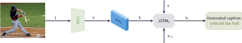
To showcase our ATPL architecture, we first study its appli-cation in a widely used image captioning task (Fang et al. 2015; He and Deng 2017). Given an input imageI, a stan-dard encoder-decoder can be employed to convert the image into an image feature vectorv, and then use the ATPL de-coder to convert it into a sentence. The overall architecture is dipected in Fig. 2.
We evaluate our approach with several baselines on the COCO dataset (COCO 2017). The COCO dataset contains 123,287 images, each of which is annotated with at least 5 captions. We use the same pre-defined splits as (Karpathy and Fei-Fei 2015; Gan et al. 2017): 113,287 images for train-ing, 5,000 images for validation, and 5,000 images for test-ing. We use the same vocabulary as that employed in (Gan et al. 2017), which consists of 8,791 words.
For the CNN of Fig. 2, we used ResNet-152 (He et al. 2016), pretrained on the ImageNet dataset. The image fea-ture vector v has 2048 dimensions. The model is imple-mented in TensorFlow (Abadi and others 2015) with the default settings for random initialization and optimization by backpropagation. In our ATPL architecture, we choose
d = 32, and the size of the LSTM hidden state to be512. The vocabulary sizeV = 8,791. ATPL uses tags as in (Gan et al. 2017).
Figure 2: Architecture of image captioning.
Table 1: Performance of the proposed ATPL model on the COCO dataset.
Methods METEOR BLEU-1 BLEU-2 BLEU-3 BLEU-4 CIDEr
NIC (Vinyals et al. 2015b) 0.237 0.666 0.461 0.329 0.277 0.855
CNN-LSTM (Gan et al. 2017) 0.238 0.698 0.525 0.390 0.292 0.889
SCN-LSTM (Gan et al. 2017) 0.257 0.728 0.566 0.433 0.330 1.012
ATPL 0.258 0.733 0.572 0.437 0.335 1.013
dataset are reported in Table 1. The widely-used BLEU (Pa-pineni et al. 2002), METEOR (Banerjee and Lavie 2005), and CIDEr (Vedantam, Lawrence Zitnick, and Parikh 2015) metrics are reported in our quantitative evaluation of the per-formance of the proposed scheme.
We can observe that, our ATPL architecture significantly outperforms all other baseline approaches across all metrics being considered. The results clearly attest to the effective-ness of the ATPL architecture. We attribute the performance gain of ATPL to the use of TPR in replace of a pure LSTM decoder, which allows the decoder to learn not only how to generate thefillersequence but also how to generate the
rolesequence so that the decoder can better understand the grammar of the considered language. Indeed, by manually inspecting the generated captions from ATPL, none of them has grammatical mistakes. We attribute this to the fact that our TPR structure enables training to be more effective and more efficient in learning the structure through the role vec-tors.
Note that the focus of this paper is on developing a Tensor Product Representation (TPR) inspired network to replace the core layers in an LSTM; therefore, it is directly compara-ble to an LSTM baseline. So in the experiments, we focus on comparison to a strong CNN-LSTM baseline. We acknowl-edge that more recent papers reported better performance on the task of image captioning. Performance improvements in these more recent models are mainly due to using better im-age features such as those obtained by Region-based Convo-lutional Neural Networks (R-CNN), or using reinforcement learning (RL) to directly optimize metrics such as CIDEr to provide a better context vector for caption generation, or using an ensemble of multiple LSTMs, among others. How-ever, the LSTM is still playing a core role in these works and we believe improvement over the core LSTM, in both performance and interpretability, is still very valuable. De-ploying these new features and architectures (R-CNN, RL, and ensemble) with ATPL is our future work.
5
Task 2: POS Tagging
In this section, we study the application of ATPL in the POS tagging task. Intuitively, given a sentence x1, ..., xT, POS
tagging is to assign a POS tag denoted aszt, for each token
xt. In the following, we first present our model using ATPL
for POS tagging, and then evaluate its performance.
5.1
ATPL POS tagging architecture
Based on TPR theory, the role vector (as well as its dual unbinding vector) contains the POS tag information of each word. Hence, we first use ATPL to compute a sequence of unbinding vectorsutwhich is of the same length as the input
sentence. Then we takeutandxtas input to a bidirectional
LSTM model to produce a sequence of POS tags.
Our training procedure consists of two steps. In the first step, we employ an unsupervised learning approach to learn how to compute ut. Fig. 3 shows a sequence-to-sequence
structure, which uses an LSTM as the encoder, and ATPL as the decoder; during the training phase of Fig. 3, the input is a sentence and the expected output is the same sentence as the input. Then we use the trained system in Fig. 3 to produce the unbinding vectorsutfor a given input sentence
x1, ..., xT.
In the second step, we employ a bidirectional LSTM (B-LSTM) module to convert the sequence ofutinto a sequence
of hidden statesh. Then we compute a vectorz1,tfrom each (xt,ht)pair, which is the POS tag at positiont. This
proce-dure is illustrated in Figure 4.
The first step follows ATPL and is straightforward. Below, we focus on explaining the second step. In particular, given the input sequenceut, we can compute the hidden states as
− →
ht,
←−
ht=BLST M(ut,
− →
ht−1, ←−
ht+1) (8)
Then, the POS tag embedding is computed as
z1,t=softmax
−→
W(xt)−→ht+
←−
W(xt)←h−t
(9)
Figure 3: Architecture for acquisition of unbinding vectors of a sentence.
Figure 4: Structure of POS tagger.
Table 2: Performance of POS Tagger.
(MANNING2017) OURPOSTAGGER
WSJ 22 WSJ 23 WSJ 22 WSJ 23 ACCURACY 0.972 0.973 0.973 0.974
−→
W(x) =−Wa→ ·diag(Wb−→ ·xt)·−Wc→ (10)
where diag(·)constructs a diagonal matrix from the in-put vector; −Wa→ ,−Wb→ ,−Wc→ are matrices of appropriate di-mensions. ←W−3,h(xt) is defined in the same manner as −→
W3,h(xt), though a different set of parameters is used. Note thatz1,tis of dimensionP, which is the total number
of POS tags. Clearly, this model can be trained end-to-end by minimizing a cross-entropy loss.
5.2
Evaluation
To evaluate the effectiveness of our model, we test it using the Penn TreeBank dataset (Marcus et al. 2017). In partic-ular, we first train the sequence-to-sequence in Fig. 3 using the sentences of Wall Street Journal (WSJ) Section 0 through Section 21 and Section 24 in Penn TreeBank data set (Mar-cus et al. 2017). Afterwards, we use the same dataset to train the B-LSTM module in Figure 4.
Once the model gets trained, we test it on WSJ Section 22 and 23 respectively. We compare the accuracy of our ap-proach against the state-of-the-art Stanford parser (Manning 2017). The results are presented in Table 2. From the table, we can observe that our approach outperforms the baseline. This confirms our hypothesis that the unsupervisely trained
unbinding vectorut indeed captures grammatical
informa-tion, so as to be used to effectively predict grammar struc-tures such as POS tags.
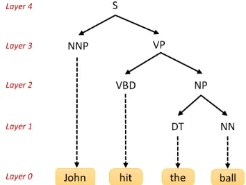
Figure 5: The parse tree of a sentence and its layers.
6
Task 3: Constituency Parsing
In this section, we briefly review the constituency parsing task, and then present our approach, which contains three component: segmenter, classifier, and creator of a parse tree. In the end, we compare our approach against the state-of-the-art approach in (Vinyals et al. 2015a).
6.1
A brief review of constituency parsing
Constituency parsing converts a natural language into its parsing tree. Fig. 5 provides an example of the parsing tree on top of its corresponding sentence. From the tree, we can label each node into layers, with the first layer (Layer 0) consisting of all tokens from the original sentence. Layerk
contains all internal nodes whose depth with respect to the closest leaf that it can reach isk.
In particular, at Layer 1 are all POS tags associated with each token. In higher layers, each node corresponds to a
Figure 6: Structure of the segmenter on Layer 2.
phrase), VP (verb phrase), (3) word-level tags such as NNP (Proper noun, singular), VBD (Verb, past tense), DT (Deter-miner), NN (Noun, singular or mass), (4) punctuation marks, and (5) special symbols such as $.
The task of constituency parsing recovers both the tree-structure and the category associated with each node. In our approach to employ ATPL to construct the parsing tree, we use an encodingzto encode the tree-structure. Our approach first generates this encoding from the raw sentence, layer-by-layer, and then predict a category to each internal node. In the end, an algorithm is used to convert the encodingz
with the categories into the full parsing tree. In the follow-ing, we present the three sub-routines.
6.2
Segmenting a sentence into a tree-encoding
We first introduce the concept of the encodingz. For each layerk, we assign a valuezk,tto each locationtof thein-put sentence. In the first layer,z1,tsimply encodes the POS
tag of input tokenxi. In a higher level,zk,t is either0 or 1. Thus the sequencezk,tforms a sequence with alternating sub-sequences of consecutive 0s and consecutive 1s. Each of the longest consecutive 0s or consecutive 1s indicate one internal node at layerk, and the consecutive positions form the substring of the node. For example, the second layer of Fig. 5 is encoded as{0,1,0,0}, and the third layer is en-coded as{0,1,1,1}.
The first component of our ATPL-based parser predicts
zk,t layer-by-layer. Note that the first layer is simply the POS tags, so we will not repeat it. In the following, we first explain how to construct the second layer’s encoding z2,t,
and then we show how it can be expanded to construct higher layer’s encodingzk,tfork≥3.
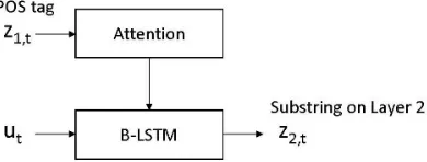
Constructing the second layerz2,t. We can viewz2,tas
a special tag over the POS tag sequence, and thus the same approach to compute the POS tag can be adapted here to computez2,t. This model is illustrated in Fig. 6.
In particular, we can compute the hidden state from the unbinding vectors from the raw sentence as before:
− →
h2,t,
←−
h2,t=BLST M(ut,
− →
h2,t−1, ←−
h2,t+1) (11)
and the output of the attention-based B-LSTM is given as below
z2,t=σs(
−→
W2(z1,t)
− →
h2,t+
←−
W2(z1,t)
←−
h2,t) (12)
where−W→2,h(z1,t)and
←−
W2,h(z1,t)are defined in the same
manner as in (10).
Figure 7: Structure of the segmenter on Layerk≥3.
Figure 8: Segmenting Layerk≥3.
Constructing higher layer’s encodingzk,t(k≥3). Now we move to higher levels. For a layerk≥3, to predictzk,t,
our model takes both the POS tag inputz1,t and the(k− 1)-th layer’s encodingzk−1,t. The high-level architecture is
illustrated in Fig. 7. Let us denote
zk,t=softmax(Jk,t)
the key difference is how to compute Jk,t. Intuitively,Jk,t
is an embedding vector corresponding to the node, whose substring contains tokenxt. Assume wordxtis in them-th
substring of Layerk−1, which is denoted bysk−1,m. Then,
the embeddingJk,tcan be computed as follows:
Jk,t= X
i∈sk−1,m −→
Wk(z1,i) − →
hk,i+
←−
Wk(z1,i) ←−
hk,i
|sk−1,m|
(13)
Here,−→hk,iand
←−
hk,i are the hidden states of BLSTM
run-ning over the unbinding vectors as before, and−Wk→ (·)and ←−
Wk(·)are defined in a similar fashion as (10). We use| · |to indicate the cardinality of a set.
The most interesting part is thatJk,t aggregates all
em-beddings computed from the substring of the previous layer
sk−1,m. Note that the set sk−1,m of indexes can be
com-puted easily fromzk−1,t. Note that many different
aggrega-tion funcaggrega-tions can be used. In (13), we choose to use the av-erage function. The process of this calculuation is illustrated in Fig. 8.
6.3
Classification of substrings
Once the tree structure is computed, we attach a category to each internal node. We employ a similar approach as pre-dictingzk,tfork≥3to predict this categoryz
(k)
t . Note that,
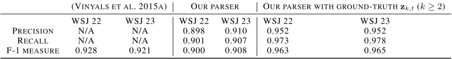
Table 3: Performance of Constituency Parser.
(VINYALS ET AL. 2015A) OUR PARSER OUR PARSER WITH GROUND-TRUTHzk,t(k≥2)
WSJ 22 WSJ 23 WSJ 22 WSJ 23 WSJ 22 WSJ 23
PRECISION N/A N/A 0.898 0.910 0.952 0.952
RECALL N/A N/A 0.901 0.907 0.973 0.978
F-1MEASURE 0.928 0.921 0.900 0.908 0.963 0.965
Figure 9: Structure of the classifier on Layerk.
computed. Thus, instead of using the encodingzk−1,tfrom
the previous layer, we use the encoding of the current layer
zk,tto predictz
(k)
t directly. This procedure is illustrated in
Fig. 9.
Similar to (13), we havez(tk) = softmax(Ek,t), where
Ek,tis computed by (∀t∈ {t:xt∈sk,m})
Ek,t= X
i∈sk,m −→
Wk(z1,i) − →
hk,i+
←−
Wk(z1,i) ←−
hk,i
|sk,m|
(14)
Here, we slightly overload the variable names. We empha-size that the parameters−W→ and←W−and the hidden states −
→
hk,iand
←−
hk,iare both independent to the ones used in (14).
Note that the main different between (14) and (13) is that, the aggregation is operated over the setsk,t, i.e., the
sub-string at layerk, rather thansk−1,t, i.e., the substring at layer
k−1. Also,Ek,t’s dimension is the same as the total number
of categories, whileJk,t’s dimension is 2.
6.4
Creating a parse tree
Once bothzk,tandz
(k)
t are constructed, we can create the
parse tree out of them using a linear-time sub-routine. Due to space limitation, we omit the details.For the example in Fig. 5, the output is (S(NNP John)(VP(VBD hit)(NP(DT the)(NN ball)))).
6.5
Evaluation
We now evaluate our constituency parsing approach against the state-of-the-art approach (Vinyals et al. 2015a) using WSJ data set in Penn TreeBank. Similar to our setup for POS tag, we train our model using WSJ Section 0 through Sec-tion 21 and SecSec-tion 24, and evaluate it on SecSec-tion 22 and 23.
Table 3 shows the performance for both (Vinyals et al. 2015a) and our proposed approach. In addition, we also eval-uate our approach assuming the tree-structure encodingzk,t
is known. In doing so, we can evaluate the performance of our classification module of the parser. Note, the POS tag is not provided.
We observe that the F-1 measure of our approach is two points worse than (Vinyals et al. 2015a); however, when the ground-truth of zk,t is provided, the F-1 measure be-comes four points higher than that reported in (Vinyals et al. 2015a), which is significant. Therefore, we attribute the somewhat lower performance of our approach to the lack of our model’s ability in effectively predicting the tree-encodingzk,t.
7
Conclusion
In this paper, we propose a novel ATPL approach to nat-ural language generation and related tasks. The model has a novel architecture motivated by insights derived from the use of Tensor Product Representations for encoding and pro-cessing symbolic structure through neural computation. In our experiments, we first evaluate the proposed model on the task of image captioning. Compared with widely adopted LSTM-based models, our proposed ATPL gives significant improvements on all major metrics including METEOR, BLEU, and CIDEr. We further observe that the unbinding vectors contain important grammatical information. This al-lows us to design an effective POS tagger and constituency parser with unbinding vectors as input, the other two NLP tasks evaluated using ATPL. Our findings reported in this paper demonstrate the effectiveness of the ATPL architec-ture as well as the underlying TPRs. In the fuarchitec-ture, we will explore the use of TPR and ATPL methods in a wider set of NLP tasks than reported in this paper, and distill further insight into structured representations of natural language.
References
Abadi, M., et al. 2015. TensorFlow: Large-scale machine learning on heterogeneous systems. Software available from tensorflow.org. Andreas, J.; Rohrbach, M.; Darrell, T.; and Klein, D. 2015. Deep compositional question answering with neural module networks. arXiv preprint arXiv:1511.027992.
Banerjee, S., and Lavie, A. 2005. Meteor: An automatic metric for mt evaluation with improved correlation with human judgments. In Proceedings of the ACL workshop on intrinsic and extrinsic evalu-ation measures for machine translevalu-ation and/or summarizevalu-ation, 65– 72. Association for Computational Linguistics.
COCO. 2017. Coco dataset for image captioning. http://mscoco. org/dataset/#download.
Fang, H.; Gupta, S.; Iandola, F.; Srivastava, S.; Deng, L.; Dollar, P.; Gao, J.; and He, X. 2015. From captions to visual concepts and back. InProc. IEEE conference on computer vision and pattern Recognition.
Gan, Z.; Gan, C.; He, X.; Pu, Y.; Tran, K.; Gao, J.; Carin, L.; and Deng, L. 2017. Semantic compositional networks for visual cap-tioning. InProceedings of the IEEE Conference on Computer Vi-sion and Pattern Recognition.
He, X., and Deng, L. 2017. Deep learning for image-to-text gener-ation: A technical overview. InIEEE Signal Processing Magazine, volume 34.
He, K.; Zhang, X.; Ren, S.; and Sun, J. 2016. Deep residual learn-ing for image recognition. InProceedings of the IEEE Conference on Computer Vision and Pattern Recognition, 770–778.
Hinton, G., et al. 2012. Deep neural networks for acoustic mod-eling in speech recognition. InIEEE Signal Processing Magazine, volume 29, 82–97.
Huang, Q.; Smolensky, P.; He, X.; Deng, L.; and Wu, D. 2017. A neural-symbolic approach to design of captcha. InAdvances in Neural Information Processing Systems Workshop.
Huang, Q.; Smolensky, P.; He, X.; Deng, L.; and Wu, D. 2018. Tensor product generation networks for deep NLP modeling. In Proc. Conf. NAACL (Long Papers), volume 1, 1263–1273. Jurafsky, D., and Martin, J. H. 2017. Speech and Language Pro-cessing. 3rd ed. draft edition edition.
Karpathy, A., and Fei-Fei, L. 2015. Deep visual-semantic align-ments for generating image descriptions. InProceedings of the IEEE Conference on Computer Vision and Pattern Recognition, 3128–3137.
Kong, L.; Alberti, C.; Andor, D.; Bogatyy, I.; and Weiss, D. 2017. Dragnn: A transition-based framework for dynamically connected neural networks.arXiv preprint arXiv:1703.04474.
Kumar, A.; Irsoy, O.; Ondruska, P.; Iyyer, M.; Bradbury, J.; Gulra-jani, I.; Zhong, V.; Paulus, R.; and Socher, R. 2016. Ask me any-thing: Dynamic memory networks for natural language processing. InInternational Conference on Machine Learning, 1378–1387. Lee, M.; He, X.; Yih, S.; Gao, J.; Deng, L.; and Smolensky, P. 2016. Reasoning in vector space: An exploratory study of question an-swering. InProc. Int. Conf. Learning Representations (ICLR). Maillard, J.; Clark, S.; and Yogatama, D. 2017. Jointly learn-ing sentence embeddlearn-ings and syntax with unsupervised tree-lstms. arXiv preprint arXiv:1705.09189.
Manning, C. 2017. Stanford parser. https://nlp.stanford.edu/ software/lex-parser.shtml.
Mao, J.; Xu, W.; Yang, Y.; Wang, J.; Huang, Z.; and Yuille, A. 2015. Deep captioning with multimodal recurrent neural networks (m-rnn). InProceedings of International Conference on Learning Representations.
Marcus, M. P.; Santorini, B.; Marcinkiewicz, M. A.; and Taylor, A. 2017. Penn treebank. https://catalog.ldc.upenn.edu/ldc99t42. Palangi, H.; Huang, Q.; Smolensky, P.; He, X.; and Deng, L. 2017. Grammatically-interpretable learned representations in deep nlp models. InAdvances in Neural Information Processing Systems Workshop.
Papineni, K.; Roukos, S.; Ward, T.; and Zhu, W.-J. 2002. Bleu: a method for automatic evaluation of machine translation. In Pro-ceedings of the 40th annual meeting on association for computa-tional linguistics, 311–318. Association for Computational Lin-guistics.
Pennington, J.; Socher, R.; and Manning, C. 2017. Stanford glove: Global vectors for word representation. https://nlp.stanford.edu/ projects/glove/.
Smolensky, P., and Legendre, G. 2006.The harmonic mind: From neural computation to optimality-theoretic grammar. Volume 1: Cognitive architecture. MIT Press.
Smolensky, P.; Lee, M.; He, X.; Yih, S.; Gao, J.; and Deng, L. 2016. Basic reasoning with tensor product representations. In arXiv:1601.02745.
Smolensky, P. 1990. Tensor product variable binding and the repre-sentation of symbolic structures in connectionist systems.Artificial intelligence46(1-2):159–216.
Tai, K. S.; Socher, R.; and Manning, C. D. 2015. Improved se-mantic representations from tree-structured long short-term mem-ory networks.arXiv preprint arXiv:1503.00075.
Toutanova, K.; Klein, D.; Manning, C. D.; and Singer, Y. 2003. Feature-rich part-of-speech tagging with a cyclic dependency net-work. InProc. NAACL, 173–180.
Vaswani, A.; Shazeer, N.; Parmar, N.; Uszkoreit, J.; Jones, L.; Gomez, A. N.; Kaiser, Ł.; and Polosukhin, I. 2017. Attention is all you need. InAdvances in Neural Information Processing Sys-tems, 6000–6010.
Vedantam, R.; Lawrence Zitnick, C.; and Parikh, D. 2015. Cider: Consensus-based image description evaluation. InProceedings of the IEEE Conference on Computer Vision and Pattern Recognition, 4566–4575.
Vinyals, O.; Kaiser, Ł.; Koo, T.; Petrov, S.; Sutskever, I.; and Hin-ton, G. 2015a. Grammar as a foreign language. InAdvances in Neural Information Processing Systems, 2773–2781.
Vinyals, O.; Toshev, A.; Bengio, S.; and Erhan, D. 2015b. Show and tell: A neural image caption generator. InProceedings of the IEEE Conference on Computer Vision and Pattern Recognition, 3156–3164.
Yogatama, D.; Blunsom, P.; Dyer, C.; Grefenstette, E.; and Ling, W. 2016. Learning to compose words into sentences with rein-forcement learning.arXiv preprint arXiv:1611.09100.