A minimally-intrusive fully 3D separated plate formulation in computational structural mechanics

(1)

R E S E A R C H A R T I C L E

Open Access

A minimally-intrusive fully 3D separated

plate formulation in computational

structural mechanics

Giacomo Quaranta

1

, Mustapha Ziane

1

, Eberhard Haug

1

, Jean-Louis Duval

1

and Francisco Chinesta

2*

*_{Correspondence:}

[email protected] 2_{PIMM, ENSAM ParisTech & ESI} GROUP Chair on Advanced Modeling and Simulation of Manufacturing Processes, 151 Boulevard de l’Hopital, 75013 Paris, France

Full list of author information is available at the end of the article

Abstract

Most of mechanical systems and complex structures exhibit plate and shell

components. Therefore, 2D simulation, based on plate and shell theory, appears as an appealing choice in structural analysis as it allows reducing the computational complexity. Nevertheless, this 2D framework fails for capturing rich physics compromising the usual hypotheses considered when deriving standard plate and shell theories. To circumvent, or at least alleviate this issue, authors proposed in their former works an in-plane–out-of-plane separated representation able to capture rich 3D behaviors while keeping the computational complexity the one of 2D simulations. In the present paper we propose an eﬃcient integration of fully 3D descriptions into existing plate software.

Keywords: Plate and Shells theories, In-plane–out-of-plane separated representations, PGD, Dynamics

Introduction

We consider the linear elastostatic problem deﬁned in the plate domain=xy×z, with xy = [0, Hx]×[0, Hy] and z = [0, Hz] in which the thickness (out-of-plane)

dimension is much lower than the other ones, i.e.HzHx, Hy.

The linear elastic behavior relating the Cauchy’s stressσand the strainεusing Voigt notation reads

σ=Cε, (1)

whereCis the elasticity matrix. The relation between strainεand displacementu(with componentsu=(u, v, w)) writes

ε= ∇su=Gu, (2)

whereG= ∇s• =1₂(∇ • +∇T•) is the symmetric gradient operator.

©The Author(s) 2019. This article is distributed under the terms of the Creative Commons Attribution 4.0 International License (http://creativecommons.org/licenses/by/4.0/), which permits unrestricted use, distribution, and reproduction in any medium, provided you give appropriate credit to the original author(s) and the source, provide a link to the Creative Commons license, and indicate if changes were made.

(2)

Considering an homogeneous and isotropic material the behavior writes

C= E

(1+ν)(1−2ν)

⎡ ⎢ ⎢ ⎢ ⎢ ⎢ ⎢ ⎢ ⎢ ⎣

1−ν ν ν 0 0 0

ν 1−ν ν 0 0 0

ν ν 1−ν 0 0 0

0 0 0 (1−₂2ν) 0 0

0 0 0 0 (1−₂2ν) 0

0 0 0 0 0 (1−₂2ν)

⎤ ⎥ ⎥ ⎥ ⎥ ⎥ ⎥ ⎥ ⎥ ⎦

. (3)

Withg(x) the body forces, the displacement ﬁeldu(x) forx ∈ is described by the linear momentum balance equation

∇ ·σ+g=0. (4)

The domain boundary∂is partitioned into Dirichlet,D, and Neumann,N, bound-aries, where displacementug and tractionsTare enforced respectively. In what follows

and without loss of generality we assumeT=0

The problem weak form associated to the strong form (4) lies in looking for the dis-placement ﬁelduverifying the Dirichlet boundary conditions such that the weak form

ε(u∗)·(C·ε(u))dx=

u∗·gdx, (5)

fulfills for any test functionu∗, with the trial and test fields defined in appropriate func-tional spaces.

Plate theory

The Reissner–Mindlin theory is based on the following fundamental hypotheses [1]: (i) on the middle plane (z=0) the in-plane displacements vanish, i.e.u(x, y, z=0)=v(x, y, z=

0)=0 that implies that points located in the middle-plane only moves vertically; (ii) the plate thickness remains unchanged; (iii) the plane stress assumption remains valid, i.e.

σzz = 0 and (v) a straight line normal to the undeformed middle plane remains straight but not necessarily orthogonal to the middle plane after deformation.

From these assumptions the displacement ﬁeld can be written as:

⎧ ⎪ ⎪ ⎨ ⎪ ⎪ ⎩

u(x, y, z)= −zθx(x, y)

v(x, y, z)= −zθy(x, y)

w(x, y, z)=w(x, y)

(6)

wherewis the vertical displacement (deﬂection) of the points on the middle plane and the rotationsθxandθycoincide with the angles followed by the normal vectors contained in the planesxzandyzrespectively in their motions.

We deﬁne the generalized displacement vector ˆu ˆ

u=[θx,θy, w]T (7) deﬁned at any point on the middle plane.

Injecting plate theory assumptions into the 3D elastostatic problem weak form, Eq. (5) reduces to the following 2D formulation

xy

ˆ

ε( ˆu∗)·Cˆˆε( ˆu)dx=

xy ˆ

(3)

whose standard ﬁnite element discretization leads to

KxyU=Bxy (9)

where for notational simplicity the hat symbol (ˆ•) is omitted. In the previous expression (9),Kxyis the stiﬀness matrix andUandBxyare the vector of the generalized displacements

and forces, the former containing nodal rotations and deﬂections and the last the dual quantities: the nodal moments and vertical nodal forces. The 3D displacement ﬁeld can be then recovered by using the relations (6).

In many cases, the complexity of the solution makes impossible the introduction of pertinent hypotheses for reducing the dimensionality of the model from 3D to 2D. In that case a fully 3D descriptions seem compulsory, and the in-plane–out-of-plane separated representations become particularly suitable.

PGD-based in-plane–out-of-plane decomposition

The in-plane–out-of-plane separated representation was applied in our former works to eﬃciently solve 3D elastic problems in plate geometries [2–4]. The elastic problem was deﬁned in a plate domain = xy ×z with (x, y) ∈ xy, xy ⊂ R2 andz ∈ z,

z ⊂R. The separated representation of the displacement ﬁeldu =(u, v, w) consists in a ﬁnite sum decomposition onN terms, each one of them consisting in the product of two unknown functions, one depending on the in-plane coordinates (x, y) and one on the out-of-plane coordinatez, i.e.:

u(x, y, z)=

⎛ ⎜ ⎜ ⎝

u(x, y, z)

v(x, y, z)

w(x, y, z)

⎞ ⎟ ⎟ ⎠≈

N

i=1

⎛ ⎜ ⎜ ⎝

ui_xy(x, y)·ui_z(z)

vi

xy(x, y)·viz(z) wi_xy(x, y)·w_zi(z)

⎞ ⎟ ⎟

⎠. (10)

Expression (10) can be written in a more compact form by using the Hadamard (component-to-component) product:

u(x, y, z)≈

N

i=1

Ui

xy(x, y)◦Uzi(z). (11)

Enriched formulations

As reported in the previous section plate kinematics can be written as a single-term separated decomposition

⎧ ⎪ ⎪ ⎪ ⎪ ⎨ ⎪ ⎪ ⎪ ⎪ ⎩

u(x, y, z)=θx(x, y)fx(z)

v(x, y, z)=θy(x, y)fy(z)

w(x, y, z)=w(x, y)fz(z)

, (12)

withfx₍_z₎_{= −}_z_,_fy₍_z₎_{= −}_z_and_fz₍_z₎₌_1.

For the sake of generality we are considering generic functionsfx(z),fy(z) andfz(z) assumed known, but than can be diﬀerent to the ones related to the standard Reissner– Mindlin plate theory, and its associated 3D kinematics given by Eq. (12). Consequently

(4)

The displacements gradient becomes

∇u= ⎛ ⎜ ⎜ ⎜ ⎜ ⎜ ⎜ ⎜ ⎜ ⎜ ⎜ ⎜ ⎜ ⎜ ⎜ ⎜ ⎜ ⎜ ⎜ ⎜ ⎜ ⎝ ∂u ∂x ∂u ∂y ∂u ∂z ∂v ∂x ∂v ∂y ∂v ∂z ∂w ∂x ∂w ∂y ∂w ∂z ⎞ ⎟ ⎟ ⎟ ⎟ ⎟ ⎟ ⎟ ⎟ ⎟ ⎟ ⎟ ⎟ ⎟ ⎟ ⎟ ⎟ ⎟ ⎟ ⎟ ⎟ ⎠ = ⎛ ⎜ ⎜ ⎜ ⎜ ⎜ ⎜ ⎜ ⎜ ⎜ ⎜ ⎜ ⎜ ⎜ ⎜ ⎜ ⎜ ⎜ ⎜ ⎜ ⎜ ⎝ ∂θx ∂x ∂θx ∂y θx ∂θy ∂x ∂θy ∂y θy ∂w ∂x ∂w ∂x w ⎞ ⎟ ⎟ ⎟ ⎟ ⎟ ⎟ ⎟ ⎟ ⎟ ⎟ ⎟ ⎟ ⎟ ⎟ ⎟ ⎟ ⎟ ⎟ ⎟ ⎟ ⎠ ◦ ⎛ ⎜ ⎜ ⎜ ⎜ ⎜ ⎜ ⎜ ⎜ ⎜ ⎜ ⎜ ⎜ ⎜ ⎜ ⎜ ⎜ ⎜ ⎜ ⎜ ⎜ ⎝ fx fx dfx₍_z₎

dz fy

fy dfy₍_z₎

dz fz fz dfz ∂z ⎞ ⎟ ⎟ ⎟ ⎟ ⎟ ⎟ ⎟ ⎟ ⎟ ⎟ ⎟ ⎟ ⎟ ⎟ ⎟ ⎟ ⎟ ⎟ ⎟ ⎟ ⎠ , (13)

that allows deﬁning the strain separated form, that taking into account its symmetry reads

ε= ⎛ ⎜ ⎜ ⎜ ⎜ ⎜ ⎜ ⎜ ⎜ ⎜ ⎜ ⎜ ⎝ ∂u ∂x ∂v ∂y ∂w ∂z ∂u ∂y+ ∂∂vx ∂u ∂z + ∂∂wx ∂v ∂z+∂∂wy

⎞ ⎟ ⎟ ⎟ ⎟ ⎟ ⎟ ⎟ ⎟ ⎟ ⎟ ⎟ ⎠ = ⎛ ⎜ ⎜ ⎜ ⎜ ⎜ ⎜ ⎜ ⎜ ⎜ ⎜ ⎜ ⎝ ∂θx ∂x ∂θy ∂y w ∂θx ∂y θx θy ⎞ ⎟ ⎟ ⎟ ⎟ ⎟ ⎟ ⎟ ⎟ ⎟ ⎟ ⎟ ⎠ ◦ ⎛ ⎜ ⎜ ⎜ ⎜ ⎜ ⎜ ⎜ ⎜ ⎜ ⎜ ⎜ ⎝ fx fy dfz dz fx dfx dz dfy dz ⎞ ⎟ ⎟ ⎟ ⎟ ⎟ ⎟ ⎟ ⎟ ⎟ ⎟ ⎟ ⎠ + ⎛ ⎜ ⎜ ⎜ ⎜ ⎜ ⎜ ⎜ ⎜ ⎜ ⎜ ⎜ ⎝ 0 0 0 ∂θy ∂x ∂w ∂x ∂w ∂y ⎞ ⎟ ⎟ ⎟ ⎟ ⎟ ⎟ ⎟ ⎟ ⎟ ⎟ ⎟ ⎠ ◦ ⎛ ⎜ ⎜ ⎜ ⎜ ⎜ ⎜ ⎜ ⎜ ⎜ ⎜ ⎝ 0 0 0 fy fz fz ⎞ ⎟ ⎟ ⎟ ⎟ ⎟ ⎟ ⎟ ⎟ ⎟ ⎟ ⎠ (14)

=1₍_{x, y}₎_◦_F1₍_z₎₊2₍_{x, y}₎_◦_F2₍_z₎_. ₍₁₅₎ In the case of a general material the Hooke tensor can also be written as

C(x, y, z)=

M

i=1

Ci

xy(x, y)◦Ciz(z). (16)

For an homogenous material we have simply

C=Ci

xy◦Ciz. (17)

whereCzis given by Eq. (3) andCxyis a tensor whose all the entries are 1,

Cxy= ⎡ ⎢ ⎢ ⎢ ⎢ ⎢ ⎢ ⎢ ⎢ ⎣

1 1 1 1 1 1

⎤ ⎥ ⎥ ⎥ ⎥ ⎥ ⎥ ⎥ ⎥ ⎦ . (18)

Taking this into consideration the method that we are going to explain can be used both for homogenous and not homogenous materials. For the sake of simplicity we are going to present it in the case where in expression (16) only one term appears in the sum, but it can be easily extended to involve more terms. The virtual work principle, expressed using a matrix notation, involves the internal work

ε∗T_σ₌_ε∗T_C_ε

= {1∗₍_{x, y}₎_◦_F1₍_z₎₊2∗₍_{x, y}₎_◦_F2₍_z₎_}T_{_C

(5)

{1₍_{x, y}₎_◦_F1₍_z₎₊2₍_{x, y}₎_◦_F2₍_z₎_}

=1∗T₍_{x, y}₎_{_C

xy(x, y)◦Cˆ11z (z)}1(x, y)+1∗T(x, y){Cxy(x, y)◦Cˆ12z (z)}

2₍_{x, y}₎₊2∗T₍_{x, y}₎_{_C

xy(x, y)◦Cˆ21z (z)}1(x, y)+2∗T(x, y)

{Cxy(x, y)◦Cˆz22(z)}2(x, y). (19)

In the previous expression matrices ˆCijz(z) results

ˆ

Cijzkl(z)=Czkl(z)F

i k(z)F

j

l(z), i, j∈[1,2] &k, l∈[1,· · ·,6]. (20)

Now, the virtual work integral reads

xy×z 2

i=1 2

j=1

i∗T₍_{x, y}₎_{_C

xy(x, y)◦Cˆijz(z)}j(x, y)dz dx dy

=

xy 2

i=1 2

j=1

i∗T₍_{x, y}₎_Dij₍_{x, y}₎j₍_{x, y}₎_{dx dy,} ₍₂₁₎

where

Dij₍_{x, y}₎₌_C

xy(x, y)◦

z ˆ

Cij

z(z)dz. (22)

Now, if we assume an approximation based on a piecewise linear interpolation on a triangular ﬁnite element, related to an in-plane mesh ofxy = ∪E

e=1exy, with the shape

functions deﬁned byN_ie(x, y), i=1,2,3;e=1,. . .,E; it results

⎧ ⎪ ⎪ ⎨ ⎪ ⎪ ⎩

θx,e₍_{x, y}₎₌_Ne

1(x, y)θ

x,e

1 +N2e(x, y)θ

x,e

2 +N3e(x, y)θ

x,e

3

θy,e₍_{x, y}₎₌_Ne

1(x, y)θ

y,e

1 +N2e(x, y)θ

y,e

2 +N3e(x, y)θ

y,e

3

we(x, y)=N₁e(x, y)we₁+N₂e(x, y)w₂e+N₃e(x, y)we₃

(23)

Using that approximation we can express vectorsi(x, y) in each elemente_{from the}

generalized nodal displacements

UeT ₌₍_θx,e

1 ,θ

y,e

1 , we1,θ2x,e,θ

y,e

2 , we2,θ3x,e,θ

y,e

3 , w3e), (24)

from

i₍₍_{x, y}₎_∈e

xy)=Bi,e(x, y)Ue, (25)

where Bi,e(x, y) contains the shape functions and theirs derivatives, according to the expressions involved in the components ofi(x, y), i=1,2.

Thus, integral (21) reads

E

e=1

Ue∗T ⎧ ⎨ ⎩ e xy 2

i=1 2

j=1

Bi,eT₍_{x, y}₎_Dij₍_{x, y}₎_Bj,e₍_{x, y}₎_{dx dy} ⎫ ⎬ ⎭Ue

=

E

e=1

Ue∗T_Ke

xyUe=U∗TKxyU. (26)

Now, if we consider the virtual work of the body forcesg(x), it involves

u∗T_g₍_x₎_, ₍₂₇₎

where without loss of generality we assume

(6)

withVT ₌₍_θx_,_θy_{, w}_{) and}_WT ₌₍_fx₍_z₎_{, f}y₍_z₎_{, f}z₍_z_{)), and the single-mode decomposition}

of the body forces given by

g(x, y, z)=G◦H, (29)

withGT =(Mx(x, y), My(x, y), T(x, y)) andHT =(hx(z), hy(z), hz(z)). The fact of consid-ering a single mode in the decomposition of the body force is not restrictive as discussed later.

The virtual work (27) can be expressed as

u∗T_g₍_x₎₌_V∗T₍_{x, y}_)ˆ_J₍_z₎_G₍_{x, y}₎_, ₍₃₀₎

where matrix ˆJreads ˆ

J_kl(z)=I_klW_k(z)H_l(z), (31) withIthe identity matrix.

Now, the integral results

xy×z

u∗T_g₍_x₎_{dz dx dy}₌

xy

V∗T₍_{x, y}₎_JG₍_{x, y}₎_{dx dy,} ₍₃₂₎

with

J=

z ˆ

J(z)dz, (33)

Integrating in the meshxy = ∪E

e=1exy,

xy

V∗T₍_{x, y}₎_JG₍_{x, y}₎_{dx dy}₌

E

e=1

e xy

Ve∗T₍_{x, y}₎_JGe₍_{x, y}₎_{dx dy,} ₍₃₄₎

whereVe(x, y) andGe(x, y) are approximated respectively from

Ve₍_{x, y}₎₌_N₍_{x, y}₎_Ue_, ₍₃₅₎

and

Ge₍_{x, y}₎₌_N₍_{x, y}₎_Re_, ₍₃₆₎

withRe containing the nodal values ofG(x, y) andN(x, y) = [N1(x, y)N2(x, y)N3(x, y)], and

Ni= ⎛ ⎜ ⎝

N_ie(x, y) 0 0

0 N_ie(x, y) 0 0 0 N_ie(x, y)

⎞ ⎟

⎠. (37)

Thus, it results

E

e=1

e xy

Ve∗T₍_{x, y}₎_JGe₍_{x, y}₎_{dx dy}₌

E

e=1

Ue∗T ⎧ ⎪ ⎨ ⎪ ⎩

e xy

NT_JN_{dx dy} ⎫ ⎪ ⎬ ⎪ ⎭R

e

=

E

e=1

Ue∗T_Ae xyRe=

E

e=1

Ue∗T_Be

xy=U∗TBxy, (38)

from which, the principle of virtual works reads

U∗T_K

(7)

Remark 1 In general the displacement decomposition within the PGD rationale involves more than a single mode, however, within the updating process, when calculating then

mode, then−1 already computed move to the right hand member, acting as generalized body force.

Remark 2 Thus, the in-plane functions determining the kinematics can be obtained from a standard plate theory software by using the elementary rigidity and forces given respec-tively byKe

xyandBexyconsidered in expression (26) and (38).

Remark 3 If tractionT=0the same procedure can be applied to treat the corresponding terms.

Calculation of the out-of plane functions

The expression of solution obtained in the previous section is given by

u(x, y, z)=

⎛ ⎜ ⎝

u(x, y, z)

v(x, y, z)

w(x, y, z)

⎞ ⎟ ⎠=

⎛ ⎜ ⎝

θx₍_{x, y}₎_fx₍_z₎ θy₍_{x, y}₎_fy₍_z₎ w(x, y)fz(z)

⎞ ⎟

⎠=V(x, y)◦W(z), (40)

where

V(x, y)=

⎛ ⎜ ⎝

θx₍_{x, y}₎ θy₍_{x, y}₎ w(x, y)

⎞ ⎟

⎠ (41)

and

W(z)=

⎛ ⎜ ⎝

fx(z)

fy(z)

fz₍_z₎ ⎞ ⎟

⎠. (42)

Now, we proceed to updated the out-of-plane functions involved inW(z) from the just calculated in-plane functionsV(x, y) by considering again the principle of virtual work

xy×z

ε(u∗)·(C·ε(u)dx=

xy×z

u∗·fdx (43)

where now in Eq. (40) the in-plane functions are assumed known and we look for the ones involved in the out-of-plane contributionW(z). Thus, the previous integral form can be integrated onxy, and then Eq. (43) reduced to a one dimensional problem inz involving as unknown functionsfx₍_z_),_fy₍_z_{) and}_fz₍_z_).

The same rationale that was previously addressed when performing the in-plane calcu-lations is considered again but now with the test functions given by

ε∗₌1₍_{x, y}₎_◦_F1∗₍_z₎₊2₍_{x, y}₎_◦_F2∗₍_z₎_, ₍₄₄₎

and

u∗(x, y, z)=V(x, y)◦W∗(z). (45)

(8)

Fig. 1 The problem taken into consideration

Table 1 Model parameters

Hx: Length in thexdirection (mm) 250

Hy: Length in theydirection (mm) 250

Hz: Length in thezdirection (mm) 250

E: Young modulus (N/m2) 2·1011

ν: Poisson coeﬃcient 0.25

Numerical results

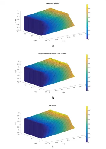
The problem taken into consideration is depicted in Fig.1. The geometrical and mechan-ical properties of the plate domain=[0, Hx]×[0, Hy]×[0, Hz] are deﬁned in Table1

On the right boundary face of the domain (the blue zone in Fig.1) a vertical traction is enforced, T = (0,0,8·109_)N_/_m2 _{and on the opposite face homogeneous Dirichlet} boundary conditions are imposed. No volumetric body forces are considered. As in the considered domain the thickness (out-of-plane) dimension is not much lower than the other ones (in-plane dimensions), the linear variation of the displacement ﬁeld along the thickness described by (2) is not more true as we can notice in Fig.2that compares the plate solution from the fully 3D solution assumed as reference. However using the just proposed minimally-intrusive fully 3D separated plate formulation we can notice how the solution is improved. Figure 3 shows the error of the solution respect to the 3D FEM solution, computed as

ξ(u)=

(u−uFEM)2dx 1 2

(uFEM)2dx 1

2

, (46)

as a function of the number of modes. The error of the plate theory solution results

ξ(uplate)=0.0633.

(9)

Fig. 2 Displacement ﬁeld using: plate theory (a), minimally-intrusive fully 3D separated plate formulation (b), 3D FEM (c)

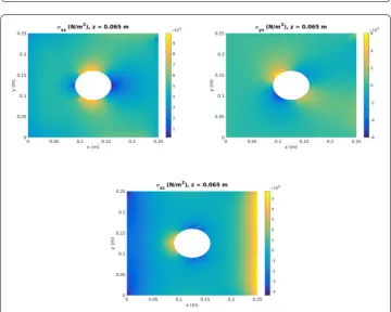
in plate theory, and to obtain the parabolic evolution around the thickness for theσxzand

σyztypical of a 3D solution (Fig.7).

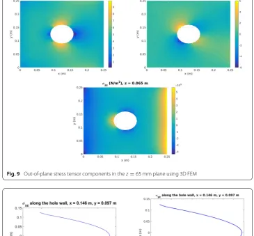
In Figs.8,9and10the same quantities are computed using a 3D ﬁnite element method, proving the good accuracy of the proposed method.

Again, in Fig.11shows the error of the solution respect to the 3D FEM solution as a function of the number of modes. The error of the plate theory solution beingξ(uplate)=

(10)

0 10 20 30 40

number of modes

0 0.01 0.02 0.03

0.04 Error respect to the 3D solution

Fig. 3 Error of the enriched solution respect to the 3D solution for diﬀerent number of modes

Extension of the method to elasto-plastic dynamics

In this section we extend the method to dynamics problem in which plastic behavior can occur. Withg(x, t) the body forces, the displacement ﬁeld evolutionu(x, t) in the domain

and time intervalt∈I=(0, T] is described by the linear momentum balance equation

ρu¨(x, t)= ∇ ·σ+g, (47)

whereρis the density (kg/m3_).

The boundary∂is decomposed according to∂=D∪Nwhere displacement and tractionsT(t) are prescribed.

The behavior relating the Cauchy’s stressσand the elastic strainεereads [5]

σ=Cεe₌_C₍_ε₋_εp₎_, ₍₄₈₎

whereCis the Hooke tensor,εis total strain andεpis the plastic strain.

The problem weak form associated with the strong form (47) results in looking for the displacement ﬁelduverifying the initial and Dirichlet boundary conditions, and fulﬁlling

ρ

u∗·u¨dx+

ε(u∗)·(C (ε(u)−εp(u)))dx=

u∗·gdx+

N

u∗·T(t)dx

(49)

for any test functionu∗in an appropriate functional space.

We consider at timetj+1the standard explicit time integration [6] (widely considered in commercial codes) given by

ρ

u∗·uj+1−2uj+uj−1

t2 dx+

ε(u∗)·

C ε(uj)−εp(uj)

dx

=

u∗·gj_d_x₊

N

u∗·Tj_d_x_, ₍₅₀₎

(11)

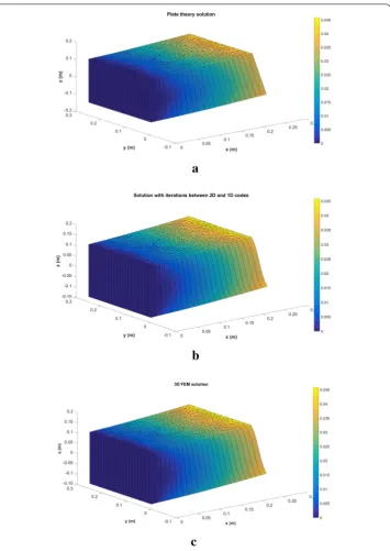
Fig. 4 Displacement ﬁeld using: plate theory (a), minimally-intrusive fully 3D separated plate formulation (b), 3D FEM (c)

ρ

u∗_·_uj+1_d_x₌_ρ

u∗_·₂_uj₋_uj−1_d_x

−t2 ⎛ ⎜ ⎝

ε(u∗)·

Cε(uj)−εp(uj)

dx+

u∗·gj_d_x₊

N

u∗·Tj_d_x ⎞ ⎟ ⎠.

(12)

Fig. 5 Out-of-plane stress tensor components around the hole using the minimally-intrusive fully 3D separated plate formulation

(13)

Fig. 7 Out-of-plane stress tensor components around the hole forx=146 mm andy=97 mm using the minimally-intrusive fully 3D separated plate formulation

(14)

Fig. 9 Out-of-plane stress tensor components in thez=65 mm plane using 3D FEM

(15)

0 5 10 15 20 25 30

number of modes

0 0.01 0.02 0.03 0.04

0.05 Error respect to the 3D solution

Fig. 11 Error of the enriched solution respect to the 3D solution for diﬀerent number of modes

Recalling (28) we can write

uj+1₍_{x, y, z}₎₌_Vj+1_◦_Wj+1_. ₍₅₂₎

Supposing the out-of-plane functions known, the left hand side term in (51) can be expressed as

u∗T_uj+1₍_x₎₌_Vj+1,∗T₍_{x, y}_)ˆ_Jj+1₍_z₎_Vj+1₍_{x, y}₎_, ₍₅₃₎ where matrix ˆJj+1reads

ˆ

Jj+1

kl (z)=IklWjk+1(z)W j+1

l (z), (54)

withIthe identity matrix. Now, the integral results

ρ

u∗·uj+1_{dz dx dy}₌

xy

Vj+1,∗T₍_{x, y}₎_Jj+1_Vj+1₍_{x, y}₎_{dx dy,} ₍₅₅₎

with

Jj+1₌

z ˆ

Jj+1₍_z₎_dz, ₍₅₆₎

Integrating in the meshxy = ∪E

e=1exy,

xy

Vj+1,∗T_Jj+1_Vj+1_{dx dy}₌

E

e=1

e xy

Vj+1,e∗T_Jj+1_Vj+1,e_{dx dy,} ₍₅₇₎

whereVj+1,e(x, y) is approximated from

Vj+1,e₍_{x, y}₎₌_N₍_{x, y}₎_Uj+1,e_, ₍₅₈₎

withN(x, y)=[N1(x, y)N2(x, y)N3(x, y)], and

Ni= ⎛ ⎜ ⎝

N_ie(x, y) 0 0

0 N_ie(x, y) 0 0 0 N_ie(x, y)

⎞ ⎟

(16)

Fig. 12 The elasto-plastic dynamical problem taken into consideration

Table 2 Model parameters

Hx: Length in the_xdirection (mm) 250

Hy: Length in the_ydirection (mm) 250

Hz: Length in the_zdirection (mm) 20

E: Young modulus (N_/m2₎ ₆_.₆₈_·₁₀10

ν: Poisson coeﬃcient 0_.35

ρ: Density (kg_/m3₎ ₂₇₀₀

Thus, it results

E

e=1

e xy

Vj+1,e∗T_Jj+1_Vj+1,e_{dx dy}₌

E

e=1

Uj+1,e∗T ⎧ ⎪ ⎨ ⎪ ⎩

e xy

NT_Jj+1_N_{dx dy}

⎫ ⎪ ⎬ ⎪ ⎭U

j+1,e

=

E

e=1

Uj+1,e∗T_Mj+1,e

xy Uj+1,e=Uj+1,∗TMjxy+1Uj+1. (60)

The diﬀerent terms at the right hand side of (51) can be treated in a similar way, as already explained for the static case, so that at each time stepjthe virtual work principle reads

Uj+1,∗T_Mj+1

xy Uj+1=Uj+1,∗TBjxy. (61)

Remark 4 As for the static case, the in-plane functions determining the kinematics can be obtained from a standard plate theory software by using the elementary mass and forces given respectively byMjxy+1,eandBj,exy.

Remark 5 Again the out-of-plane functions can be obtained in a similar manner as already explained in the static case.

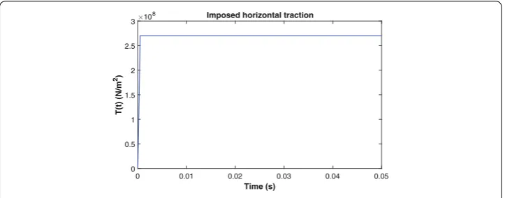
For evaluating the performances of the method we consider the problem deﬁned in Fig.12. The geometrical and mechanical properties of the plate domain are deﬁned in Table2. On the right boundary face of the domain (the blue zone in Fig.12) an horizontal traction is enforced, T = (2.7·108,0,0)N/m2and on the opposite face homogeneous Dirichlet boundary conditions are imposed. No volumetric body forces are considered. For the sake of simplicity, we use the Von Mises criterion [7], assuming a Krupkowski isotropic hardening [8] given by the formula:

¯

σ =Kε¯0+εp¯

p

(62)

where ¯ε0=0.008 is the initial equivalent plastic strain, ¯εpis the equivalent plastic strain,

(17)

0 0.01 0.02 0.03 0.04 0.05

Time (s)

0 0.5 1 1.5 2 2.5 3

T(t) (N/m

2)

108 Imposed horizontal traction

Fig. 13 Horizontal loading for the elasto-plastic dynamical problem

Fig. 14 Displacement ﬁeld using the three methods fort=0.1 ms andt=0.5 ms

(18)

Fig. 15 Displacement ﬁeld using the three methods fort=1 ms andt=5 ms

⎧ ⎪ ⎪ ⎨ ⎪ ⎪ ⎩

u(x, y, z)=u0(x, y)−zθx(x, y)

v(x, y, z)=v0(x, y)−zθy(x, y)

w(x, y, z)=w0(x, y)

(63)

where u0, v0 and w0 are the displacements of the points on the middle plane along

x, y and z respectively and the rotations θx and θy coincide with the angles fol-lowed by the normal vectors contained in the planes xz and yz respectively in their motions.

Again the solution computed using the proposed method is able to get a 3D behavior (as the one of the 3D FEM solution) with the striction along the thickness in the zone with a smaller section, which is typical of a 3D plastic solution.

Conclusions

(19)

Fig. 16 Displacement ﬁeld using the three methods fort=10 ms andt=30 ms

1D problems extremely simple and cheap, is externalized and ensured by a function called by the plate solver.

The diﬀerent numerical examples prove the procedure eﬃciency that allows computing 3D solutions while keeping the computational cost the one characteristic of standard 2D plate and shell calculations.

Authors’ contributions

GQ, MZ, EH, JLD and FC authors participated in the deﬁnition of techniques and algorithms. All authors read and approved the ﬁnal manuscript.

Author details

1_{ESI Group, Parc Icade, Immeuble le Seville, 3 bis, Saarinen, CP 50229, 94528 Rungis Cedex, France,}2_{PIMM, ENSAM} ParisTech & ESI GROUP Chair on Advanced Modeling and Simulation of Manufacturing Processes, 151 Boulevard de l’Hopital, 75013 Paris, France.

Acknowledgements

Authors acknowledge the support of the ESI Group through its research chair at ENSAM ParisTech.

Funding

This project has received funding from the European Union’s Horizon 2020 research and innovation programme under the Marie Skłodowska-Curie Grant Agreement No. 675919.

Availability of data and materials

Interested reader can contact authors.

Competing interests

(20)

Appendix A: Calculation of the out-of plane functions in a minimally-intrusive manner

We write the virtual work principle

ε∗T_σ₌_ε∗T_C_ε

= {1₍_{x, y}₎_◦_F1∗₍_z₎₊2₍_{x, y}₎_◦_F2∗₍_z₎_}T_{_C

xy(x, y)◦Cz(z)} {1₍_{x, y}₎_◦_F1₍_z₎₊2₍_{x, y}₎_◦_F2₍_z₎_}

=F1∗T₍_{x, y}₎_{_C_ˆ11

xy(x, y)◦Cz(z)}F1(x, y)+F1∗T(x, y){Cˆ12xy(x, y)◦Cz(z)}

F2₍_{x, y}₎₊_F2∗T₍_{x, y}₎_{_C_ˆ21

xy(x, y)◦Cz(z)}F1(x, y)+F2∗T(x, y) {_Cˆ22

xy(x, y)◦Cz(z)}F2(x, y). (64)

In the previous expression matrices ˆCijxy(x, y) results

ˆ

Cij

xykl(x, y)=Cxykl(x, y)

i k(x, y)

j

l(x, y), i, j∈[1,2] & k, l∈[1,· · ·,6]. (65)

Now, the virtual work integral reads

xy×z 2

i=1 2

j=1

Fi∗T₍_z₎_{_C_ˆij

xy(x, y)◦Cz(z)}Fj(z)dz dx dy

=

z 2

i=1 2

j=1

Fi∗T₍_z₎_Pij₍_z₎_Fj₍_z₎_dz, ₍₆₆₎

where

Pij₍_z₎₌_C z(z)◦

xy ˆ

Cij

xy(x, y)dx dy. (67)

Now, if we assume for instance an approximation based on piecewise linear interpola-tions on the 1D ﬁnite element mesh ofz = ∪Q_q₌₁qz, with the shape functions deﬁned

byN_iq(z), i=1,2; q=1,. . .,Q; it results

⎧ ⎪ ⎪ ⎨ ⎪ ⎪ ⎩

fx,q(z)=N₁q(z)f₁x,q+N₂q(z)f₂x,q

fy,q(z)=N₁q(z)f₁y,q+N₂q(z)f₂y,q

fz,q(z)=N₁q(z)f₁z,q+N₂q(z)f₂z,q

(68)

Using that approximation we can express vectorsFi₍_z_{) in each element}q zfrom

LqT ₌₍_fx,q

1 , f

y,q

1 , f

z,q

1 , f

x,q

2 , f

y,q

2 , f

z,q

2 ), (69)

and

Fi₍_z_∈q

z)=Ti,q(z)Lq, (70)

(21)

Thus, integral (66) reads

Q

q=1

Lq∗T ⎧ ⎪ ⎨ ⎪ ⎩ q z 2

i=1 2

j=1

Ti,qT₍_z₎_Pij₍_z₎_Tj,q₍_z₎_dz ⎫ ⎪ ⎬ ⎪ ⎭L q = Q

q=1

Lq∗T_Kq

zLq=L∗TKzL. (71)

The virtual work (27) of the body forces can be expressed as

u∗T_g₍_x₎₌_W∗T₍_z_{) ˆ}_O₍_{x, y}₎_H₍_z₎_, ₍₇₂₎

where matrix ˆOreads ˆ

Okl(x, y)=IklVk(x, y)Gl(x, y), (73)

withIthe identity matrix. Now, the integral results

xy×z

u∗T_g₍_x₎_{dz dx dy}₌

z

W∗T₍_z₎_OH₍_z₎_dz, ₍₇₄₎

with

O=

xy ˆ

O(x, y)dx dy, (75)

Integrating in the meshz= ∪Q_q₌₁qz,

z

W∗T₍_z₎_OH₍_z₎_dz₌

Q

q=1

q z

Wq∗T₍_z₎_OHq₍_z₎_dz, ₍₇₆₎

whereWq(z) andHq(z) are approximated respectively from

Wq₍_z₎₌_S₍_z₎_Lq_, ₍₇₇₎

and

Hq₍_z₎₌_S₍_z₎_Mq_, ₍₇₈₎

withMqcontaining the nodal values ofH(z) andS(z)=[N1(z)N2(z)], and

Ni=

N_iq(z) 0 0 N_iq(z)

. (79)

Thus, it results

Q

q=1

q

Wq∗T₍_z₎_OHq₍_z₎_dz₌

Q

q=1

Lq∗T ⎧ ⎪ ⎨ ⎪ ⎩ q z

ST_OS_dz ⎫ ⎪ ⎬ ⎪ ⎭M q = Q

q=1

Lq∗T_Aq zMq=

Q

q=1

Lq∗T_Bq

z =L∗TBz, (80)

from which, the principle of virtual works reads

L∗T_K

zL=L∗TBz. (81)

Thus, the out-of-plane functions determining the kinematics can be obtained from a standard 1D software by using the elementary rigidity and forces given respectively byK_zq andBq_z considered in expression (71) and (80).

(22)

References

1. Oñate E. Structural analysis with the ﬁnite element method. Linear statics, vol. 2., Beams, plates and shellsNew York: McGraw-Hill; 2010.

2. Bognet B, Bordeu F, Chinesta F, Leygue A, Poitou A. Advanced simulation of models deﬁned in plate geometries: 3D solutions with 2D computational complexity. Comput Methods Appl Mech Eng. 2012;201:1–2.

3. Bognet B, Leygue A, Chinesta F. Separated representations of 3D elastic solutions in shell geometries. Adv Model Simul Eng Sci. 2014;1(1):4.

4. Quaranta G, Bognet B, Ibañez R, Tramecon A, Haug E, Chinesta F. A new hybrid explicit/implicit in-plane-out-of-plane separated representation for the solution of dynamic problems deﬁned in plate-like domains. Comput Struct. 2018;210:135–44.

5. Owen DRJ, Hinton E. Finite elements in plasticity: theory and practice. Swansea: Pine Ridge Press; 1980. 6. Bathe KJ. Finite element procedures, vol. 2. 2006.

7. Mises RV. Mechanik der festen Krper im plastisch-deformablen Zustand. Nachrichten von der Gesellschaft der Wis-senschaften zu Gottingen. Mathematisch-Physikalische Klasse. 1913;1913:582–92.

8. Siser M, Slota J. Material Model of AW 5754 H11 Al alloy for numerical simulation of deep drawing process, vol. 20. 2016.

9. Wilkins ML, Streit RD, Reaugh JE. Cumulative-strain-damage model of ductile fracture: simulation and prediction of engineering fracture tests. San Leandro: Science Applications; 1980.

Publisher’s Note