www.adv-radio-sci.net/14/175/2016/ doi:10.5194/ars-14-175-2016
© Author(s) 2016. CC Attribution 3.0 License.
Delayed response of the global total electron content to
solar EUV variations
Christoph Jacobi1, Norbert Jakowski2, Gerhard Schmidtke3, and Thomas N. Woods4 1Leipzig Institute for Meteorology, Universität Leipzig, Stephanstr. 3, 04103 Leipzig, Germany 2German Aerospace Center, Kalkhorstweg 53, 17235 Neustrelitz, Germany
3Fraunhofer-Institut für Physikalische Messtechnik (IPM), Heidenhofstraße 8, 79110 Freiburg, Germany 4LASP, University of Colorado, 3665 Discovery Dr., Boulder, CO 80303, USA
Correspondence to:Christoph Jacobi ([email protected])
Received: 27 November 2015 – Revised: 24 February 2016 – Accepted: 4 April 2016 – Published: 28 September 2016
Abstract.The ionospheric response to solar extreme ultravi-olet (EUV) variability during 2011–2014 is shown by simple proxies based on Solar Dynamics Observatory/Extreme Ul-traviolet Variability Experiment solar EUV spectra. The daily proxies are compared with global mean total electron con-tent (TEC) computed from global TEC maps derived from Global Navigation Satellite System dual frequency measure-ments. They describe about 74 % of the intra-seasonal TEC variability. At time scales of the solar rotation up to about 40 days there is a time lag between EUV and TEC variability of about one day, with a tendency to increase for longer time scales.
1 Introduction
The solar extreme ultraviolet (EUV) radiation varies on dif-ferent time scales, including the 27-day Carrington rotation as one of the primary sources of variability at the intra-seasonal time scale. Consequences are strong changes of the Total Electron Content (TEC), which is the vertically inte-grated electron density of the ionosphere/plasmasphere sys-tems, often given in terms of TEC Units (TECU, 1 TECU = 1016electrons m−2). The majority of the electrons are found in the ionospheric F layer where, according to simple the-ory based on an oxygen dominated thermosphere, the elec-tron density is proportional to the ionization rate. Therefore, TEC variability is a coarse estimate for ionization as well, so that indices describing ionization may be compared against ionospheric TEC or, in turn, these indices may be used to provide a first estimate of ionospheric TEC. In addition to
the frequently used F10.7 (solar radio flux at 10.7 cm) in-dex measured by the National Research Council of Canada (NRCC, 2014), proxies based on solar EUV, like E10.7 (To-biska, 2001) are used to characterize the solar variability and its influence on the atmosphere/ionosphere. It has been found that other proxies based on EUV measurements or combina-tion of proxies may characterize ionospheric variacombina-tions bet-ter (e.g. Maruyama, 2010). Also using the MgII index has been found to be a better representation when used in atmo-spheric models or to describe the ionosphere (Thuillier and Bruinsma, 2001; Maruyama, 2010). Unglaub et al. (2011, 2012) have introduced a proxy, termed EUV-TEC, which is based on the vertically and globally integrated primary ion-ization rates. It has been calculated from spectral EUV fluxes measured by the Solar EUV Experiment (SEE) on board the Thermosphere Ionosphere Mesosphere Energetics and Dy-namics (TIMED) satellite (Woods et al., 2000, 2005). Using data of about one decade, Unglaub et al. (2011, 2012) re-confirmed that ionization calculations based on the measured spectra describe the TEC variability better than e.g. F10.7.
Figure 1.Time series of daily integrated EUV fluxes (6–106 nm, red) from SDO/EVE and daily averaged global mean TEC (green).
O that has been created via O2photo-dissociation in the spec-tral region of the Schumann–Runge continuum from 135 to 176 nm. Since the major F region ionization is proportional to O, these results were consistent with the observed delayed ionospheric ionization response.
In this paper, we shall make an attempt to analyze the ionospheric delay based on datasets that represent solar EUV variability. In particular, we will investigate the time lag at different time scales between about 2 weeks and 3 months. We shall use integrated EUV-fluxes from the Extreme Ul-traviolet Variability Experiment (EVE) on the Solar Dynam-ics Observatory (SDO), the EUV-TEC proxy based on the SDO/EVE spectra and the NRLMSISE-00 model (Picone et al., 2002). We shall use data from 2011 through early spring 2014, and analyze the correlation between EUV proxies and global TEC variability, as well as the ionospheric delay at different time scales.
2 Data and analysis
SDO was launched on 11 February 2010 (Pesnell et al., 2012), and data are available from 1 May 2010. EVE on-board SDO measures the solar EUV irradiance from 0.1 to 106 nm with a spectral resolution of 0.1 nm, a temporal ca-dence of ten seconds, and an accuracy of 20 % (Woods et al., 2012). The in-flight calibration for EVE includes daily measurements with redundant foil filters and on-board flat-field lamps and annual underflight calibration rocket flights. Diode-based broadband channels are also used to monitor the performance and drift of the high-resolution spectrographs.
For comparison of EUV parameters with ionospheric vari-ability, daily mean global mean TEC values have been cal-culated based on International Global Navigation Satellite System Service (IGS) TEC maps (Hernandez-Pajares et al., 2009) provided by CDDIS (2015), and they will be used
violet (FUV) irradiance up to about 130 nm also contributes to ionization, but its contribution is not included in the inte-grated EUV band because their ionization contributions are primarily below the ionosphere F layer that is most impor-tant for TEC. EUV-TEC is calculated from the satellite-borne EUV measurements assuming a model atmosphere that con-sists of four major atmospheric constituents. Regional num-ber densities of the background atmosphere are taken from the NRLMSISE-00 model (Picone et al., 2002). This model uses the F10.7 flux as daily input, and additionally as 81-day mean. Since the main input to EUV-TEC is the solar EUV, it is strongly correlated to the integrated EUV flux. The corre-lation coefficient isr=0.997.
The original SDO/EVE spectra integrated from 6–106 nm and the EUV-TEC proxy are subsequently used for compar-ison with global TEC. Because the annual cycle of global TEC and ionization is different, especially owing to the semi-annual cycle in TEC, we here consider the seasonal time scale up to 3 months only. Therefore the data have been high-pass filtered using a FFT filter with a cut-off period of 3 months.
To allow comparison, the datasets were normalized by subtracting the mean and dividing by the standard devia-tion using the data from 16 March 2011 through 11 Febru-ary 2014 (approx. Carrington rotations 2108–2146). The mean values and standard deviations are 1.438±0.078× 10¹⁹ions m−2 for the EUV-TEC ionization rates, 4.252± 0.238 mWm−2 for SDO/EVE fluxes, and 24.9±2.1 TECU for global TEC. The normalized time series are shown in Fig. 2. The curves are offset vertically by 2 with respect to each other. One can see that the variability, in particular the amplitude of the 27-day solar rotation, of TEC and EUV fluxes and EUV-TEC is very similar.
Figure 2.Time series of EUV-TEC (black), SDO/EVE integrated flux (red) and daily averaged global mean TEC (green), filtered us-ing a high-pass filter with cut-off period of 3 months and normal-ized by their mean and standard deviation. The curves are offset vertically with respect to each other.
information has been added to calculate EUV-TEC. We shall discuss this below.
Figure 4 shows Morlet wavelet spectra of SDO/EVE inte-grated EUV fluxes (left panel) and daily mean global mean TEC (right panel). Data have been normalized and low-pass filtered as in Fig. 2. The main variation is clearly near 27 days, but there is also some power at longer time scales, although this is only intermittent.
Figure 5 shows an example of time series of SDO/EVE integrated EUV fluxes and global TEC, which have fur-ther been filtered using a Lanczos bandpass filter with 100 weights and cut-off periods of 25 and 29 days, so that the time series represents the respective variability within the 27-day solar cycle. We note a delay of TEC with respect to solar variability. To systematically investigate the delay at differ-ent time scales, we now filtered the time series in differdiffer-ent period bands, and the cut-off periods of the Lanczos filter were chosen in such a way that each period band ranges over 4 days, while the center of the period band was shifted from 4 to 88 days. For each pair of filtered time series, i.e. for each time scale (which was defined as the center of the respec-tive period window), the cross-correlation coefficients were calculated. The results are shown as contour lines in Fig. 6; the line with a cross correlation ofr=0.8 is highlighted. On the ordinate the time lag is given in degrees, and 360◦ corre-sponds to the respective time scale on the abscissa. Dashed blue lines indicate lags of 0, 1, 2, and 3 days, respectively. Positive lag values indicate that EUV variations lead TEC ones. Solid light blue dots are added that show the SDO/EVE flux time lag with maximum correlation which can, how-ever, only be provided at an accuracy of one day. The black dots show these maxima again, but now calculated with using
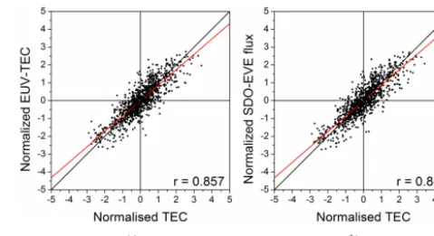
Figure 3. EUV-TEC (a), and integrated SDO/EVE flux (b) vs. global mean TEC. Data have been normalized and filtered as in Fig. 2.
EUV-TEC instead of integrated EUV fluxes. Figure 6 shows that at short time scales of few days, the correlation is weak and the shown lag values are not significant. At time scales of the solar rotation, the strongest correlation is found and so-lar variations lead global TEC by about one day. For slightly longer time scales, the delay increases, however, the power at the 30–40 day time scale is not strong as is shown in the wavelets in Fig. 4. For EUV-TEC, the lag increases to about 2 days for time scales around 2 months, but relative to the time scale the delay is not longer than for the 27-day cycle.
At first glance the difference in lag at time scales > 55 days may contradict the strong correlation of integrated EUV fluxes and EUV-TEC, However, at these time scales the correlation coefficients are still large (betweenr=0.8 and
r=0.85), but the amplitudes are smaller (see Fig. 4) so that this period range does not contribute very much to the total correlation. Furthermore, as can be seen in Fig. 6, the change ofrwith lag is small near the maximum and the difference of correlation at lag 1 or 2 days is therefore small as well (bothr
are > 99 % of the maximum lag at the respective time scale). A further effect may be due to the used resolution of 1 day, and the difference of the real lags may actually be smaller than 1.
res-Figure 4.Morlet wavelet spectra of(a)SDO/EVE integrated EUV fluxes and(b)daily mean global mean TEC. Data have been normalized and filtered as in Fig. 2.
Figure 5.Example of normalized SDO/EVE integrated EUV fluxes and global mean TEC, additionally filtered in the 25–29 days period range.
olution used here, these findings cannot be considered as a proof for this behavior of the ionospheric delay, they may in-dicate that the processes leading to the delay at different time scales may be different.
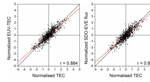
We have made an attempt to include the ionospheric delay shown in Figs. 6 and 7 into the EUV and EUV-TEC time se-ries. The time series had been filtered in the respective time ranges, the shifted by the delay (0–2 days), and then the fil-tered series had been added up again. As expected, the corre-lation increases, namely tor=0.88 for EUV-TEC and 0.89 for SDO/EVE EUV, respectively. We note that EUV-TEC de-scribes global TEC fluctuations still a little worse than the EUV fluxes do. We also made first analyses of the EUV-TEC proxy using an index based on SDO/EVE EUV fluxes integrated from 6–106 nm instead of F10.7 in NRLMSISE-00. This leads to a slightly stronger correlation of EUV-TEC with TEC, but still it is not stronger than using EUV directly. Clearly, EUV-TEC is a very simple proxy. A much more sophisticated parameterization for use in general circulation models have been constructed by Solomon and Qian (2005).
Figure 6. Cross-correlation coefficients between filtered global TEC and SDO/EVE integrated EUV fluxes. The time scale on the abscissa defines the center of the 4-day period band of the respec-tive filter. On the ordinate the time lag is given in degrees, and 360◦ corresponds to the respective time scale on the abscissa. Positive lag values indicate that EUV variations lead TEC ones. The dashed blue lines indicate lags of 0, 1, 2, 3 days as indicated on top of the figure. The light blue dots show the lag with maximum correlation at an accuracy of one day. The black dots show these maxima, but calculated using EUV-TEC instead of integrated EUV fluxes.
4 Conclusions
Figure 7.As in Fig. 6, but shown is the ratio of the cross-correlation coefficient and the one at the lag of maximum correlation.
It should, however, be stated here that the EUV fluxes and the ionization rates calculated by the EUV-TEC model rep-resent only a coarse description of global TEC, and they are not well suited to describe ionization e.g. in circula-tion models. A parameterizacircula-tion of ionizacircula-tion and dissoci-ation rates including photoelectron effects using solar spec-tral measurements or models has been presented by Solomon and Qian (2005). When used as a TEC proxy, EUV-TEC does not account for dynamics, secondary ionization, or ionization through particle precipitation. It does not take into account effects of ionospheric storms, which are a challenge for TEC forecast (Borries et al., 2015). Nevertheless, the integrated EUV flux or EUV-TEC describes TEC variations well, espe-cially at the time scale of the solar rotation.
Obviously, the results presented here are preliminary. We used daily EUV spectra and daily and globally averaged TEC, which gives only coarse values for the ionospheric de-lay. Furthermore, F10.7 is observed at local noon and this may lead to a bias between F10.7 used in NRLMSISE-00 and daily TEC. TEC maps are available at higher temporal resolution, and EUV fluxes at least for some spectral bands are also available e.g. from the Solar and Heliospheric Ob-servatory/Solar Extreme Ultraviolet Monitor (SOHO/SEM, Judge et al., 1998) or the Geostationary Operational Envi-ronmental Satellites (GOES). This provides the possibility to study ionospheric delay in higher temporal resolution and spatially resolved. However, for the calculation of the EUV-TEC index spectral resolution is required, so that this would only provide a guidance for further improvements. There are still some further shortcomings of EUV-TEC. One aspect is probably the use of F10.7 in the NRLMSISE-00 atmosphere model used, so that EUV-TEC in this version is based on EUV spectra and F10.7. First preliminary results using the EUV-TEC proxy including NRLMSISE-00 based on EUV fluxes showed slightly better correlation with TEC, however, still gave slightly weaker correlation than using EUV inte-grated fluxes alone.
Figure 8.As in Fig. 3, but with EUV-TEC and SDO/EVE integrated fluxes shifted according to the delay as shown in Figs. 6 and 7.
Another aspect is that we completely neglect the thermo-sphere and its dynamics in the analysis. If the delay should be caused by dynamical processes as suggested by Jakowski et al. (1991), it is at least partly driven by FUV radiation and therefore the spectra used here are not necessarily suf-ficient to describe the variability. Further analyses, therefore will take this in to account, e.g. by using the MgII index in-stead of EUV, or in a combination.
Code availability
The EUV-TEC model can be obtained from the correspond-ing author on request. The code includes the NRLMSIS-00 model provided by CCMC via ftp://hanna.ccmc.gsfc.nasa. gov/pub/modelweb/atmospheric/msis/nrlmsise00/.
Data availability
IGS gridded TEC data has been provided via NASA through ftp://cddis.gsfc.nasa.gov/gps/products/ionex/. Daily F10.7 solar proxies have been provided by NGDC via http://www. ngdc.noaa.gov/stp/space-weather/solar-data/solar-features/ solar-radio/noontime-flux/penticton/penticton_observed/. The daily SDO/EVE version 5 spectra are available at LASP through http://lasp.colorado.edu/eve/data_access/ evewebdataproducts/merged/.
Acknowledgements. The original version of the EUV-TEC model has been written by C. Unglaub, Leipzig. We acknowledge support from the German Research Foundation (DFG) and Universität Leipzig within the program of Open Access Publishing.
Edited by: M. Förster
tal Electron Content, J. Geophys Res.-Space, 120, 3175–3186, doi:10.1002/2015JA020988, 2015.
CDDIS: GNSS Atmospheric Products, available at: http://cddis.nasa.gov/Data_and_Derived_Products/GNSS/ atmospheric_products.html, last access: 19 June 2015.
Hernandez-Pajares, M., Juan, J. M., Sanz, J., Orus, R., Garcia-Rigo, A., Feltens, J., Komjathy, A., Schaer, S. C., and Krankowski, A.: The IGS VTEC maps: a reliable source of ionospheric informa-tion since 1998, J. Geod., 83, 263–275, 2009.
Jakowski, N., Fichtelmann, B., and Jungstand, A.: Solar activity control of ionospheric and thermospheric processs, J. Atmos. Terr. Phys., 53, 1125–1130, 1991.
Judge, D. L., McMullin, D. R., Ogawa, H. S., Hovestadt, D., Klecker, B., Hilchenbach, M., Möbius, E., Canfield, L. R., Vest, R. E., Watts, R., Tarrio, C., Kühne, M., and Wurz, P.: First Solar EUV Irradiances Obtained from SOHO by the Celias/Sem, Solar Phys., 177, 161–173, 1998.
LASP: Extreme ultraviolet Variability Experiment – Data, avail-able at: http://lasp.colorado.edu/home/eve/data/data-access/, last access: 14 July 2015.
Lee, C.-K., Han, S.-C., Bilitza, D., and Seo, K.-W.: Global charac-teristics of the correlation and time lag between solar and iono-spheric parameters in the 27-day period, J. Atmos. Sol.-Terr. Phys., 77, 219–224, doi:10.1016/j.jastp.2012.01.010, 2012. Maruyama, T.: Solar proxies pertaining to empirical ionospheric
total electron content models, J. Geophys. Res., 115, A04306, doi:10.1029/2009JA014890, 2010.
NRCC: F10.7 radio flux index, available at: http://www.ngdc.noaa. gov/stp/space-weather/solar-data/solar-features/solar-radio/ noontime-flux/, last access: 24 September 2014.
doi:10.5194/angeo-19-219-2001, 2001.
Tobiska, W. K.: Validating the solar EUV Proxy, E10.7, J. Geophys. Res., 106, 29969–29978, doi:10.1029/2000JA000210, 2001. Unglaub, C., Jacobi, Ch., Schmidtke, G., Nikutowski, B., and
Brun-ner, R.: EUV-TEC proxy to describe ionospheric variability using satellite-borne solar EUV measurements: first results, Adv. Space Res., 47, 1578–1584, doi:10.1016/j.asr.2010.12.014, 2011. Unglaub, C., Jacobi, Ch., Schmidtke, G., Nikutowski, B., and
Brun-ner, R.: EUV-TEC proxy to describe ionospheric variability us-ing satellite-borne solar EUV measurements, Adv. Radio Sci., 10, 259–263, doi:10.5194/ars-10-259-2012, 2012.
Woods, T. N., Bailey, S., Eparvier, F., Lawrence, G., Lean, J., Mc-Clintock, B., Roble, R., Rottmann, G. J., Solomon, S. C., To-biska, W. K., and White, O. R.: TIMED Solar EUV Experiment, Phys. Chem. Earth Pt. C, 25, 393–396, 2000.
Woods, T. N., Eparvier, F., Bailey, S., Chamberlin, P., Lean, J., Rottmann, G. J., Solomon, S. C., Tobiska, W. K., and Woodraska, D. L.: Solar EUV Experiment (SEE): Mission overview and first results, J. Geophys. Res., 110, A01312, doi:10.1029/2004JA010765, 2005.