Reliability and Availability Models of Belt Drive Systems Considering Failure Dependence

ORIGINAL ARTICLE

Reliability and Availability Models of Belt

Drive Systems Considering Failure Dependence

Peng Gao

_{, Liyang Xie}

_{and Jun Pan}

Abstract

Conventional reliability models of belt drive systems in the failure mode of fatigue are mainly based on the static stress strength interference model and its extended models, which cannot consider dynamic factors in the opera-tional duration and be used for further availability analysis. In this paper, time-dependent reliability models, failure rate models and availability models of belt drive systems are developed based on the system dynamic equations with the dynamic stress and the material property degradation taken into account. In the proposed models, dynamic failure dependence and imperfect maintenance are taken into consideration. Furthermore, the issue of time scale inconsist-ency between system failure rate and system availability is proposed and addressed in the proposed system avail-ability models. Besides, Monte Carlo simulations are carried out to validate the established models. The results from the proposed models and those from the Monte Carlo simulations show a consistency. Furthermore, the case studies show that the failure dependence, imperfect maintenance and the time scale inconsistency have significant influ-ences on system availability. The independence assumption about the belt drive systems results in underestimations of both reliability and availability. Moreover, the neglect of the time scale inconsistency causes the underestimate of the system availability. Meanwhile, these influences show obvious time-dependent characteristics.

Keywords: Availability, Reliability, Belt drive, Failure dependence, Time scale inconsistency

© The Author(s) 2019. This article is distributed under the terms of the Creative Commons Attribution 4.0 International License (http://creat iveco mmons .org/licen ses/by/4.0/), which permits unrestricted use, distribution, and reproduction in any medium, provided you give appropriate credit to the original author(s) and the source, provide a link to the Creative Commons license, and indicate if changes were made.

1 Introduction

As an important form of mechanical transmission, belt drive systems are widely used in automotive, robotics, agricultural machinery and home appliances to transfer movement and power [1–3]. The merits of the belt drive systems include long lifetime, low cost and the capability of transferring motion over a long distance. In recent years, more and more requirements for high reliability and safety of belt drive systems have been developed, due to their increasing usage in mechanical products with the demands of high accuracy, high speed, high power, long lifetime and low noise. Therefore, it is imperative to develop accurate availability and reliability models with the working mech-anism taken into consideration in terms of the structure, stress and material parameters of belt drive systems.

In the last few decades, a great deal of innovative work has been carried out to investigate the availability, reliabil-ity and maintenance and of belt drive systems. For instance, Ref. [4] analyzed the failure mode of belt drives and pro-posed a method for reliability-based design of belt drives. An et  al. [5] considered the variation of lengths among individual belts in a multiple V-belt drive associated with its influences on the transmitted power. Moreover, reliabil-ity models were developed by modeling the multiple V-belt drive as a multistate weighted k-out-of-n system based on the universal generating function technique. Bai and Mu [6] presented a dynamic reliability model of belt drive systems in mines by using the three-parameter Weibull distribution to process the system failure data. A reliability-based optimal design method of V-belt drive was proposed by Gong et  al. [7] in which the number of the belt were adopted as the objective function and the system reliable as the constraint condition. Sun et al. [8] provided a method for lifetime estimation of V-belt drive under different reli-ability level and numerical examples were given to validate the proposed method. Mazurkiewicz [9] pointed out that

Open Access

*Correspondence: gaogaopeng@163.com

1 _{School of Mechanical Engineering, Liaoning Shihua University,} Fushun 113001, China

the system availability depended on a variety of factors including design, manufacturing, industrial diagnosis and maintenance. Furthermore, a computer-aided maintenance method was presented by the author. These papers pro-vided a sound theoretical basis for availability and reliability estimation of belt drive systems.

In existing references, the slipping failure and the fatigue failure are considered as the two main failure modes of belt drive systems. In this paper, we are focused on the fatigue failure model of belt drive systems. In this failure mode, the well-known stress-strength interference (SSI) model as well as its extended models is always adopted to calculate the system reliability, which is essentially a static reliability model. Moreover, great progress has been made in the estimation methods of system availability and main-tainability, which provides the possibility for quantitative availability evaluation of mechanical system when consid-ering different maintenance behaviors and maintenance strategies. For instance, Sahraoui et  al. [10] proposed a method for maintenance planning of pipelines in the fail-ure mode of corrosion considering imperfect inspections. Dehghanian et al. presented a framework for maintenance of power distribution systems based on reliability analysis. The implementation procedures for system maintenance were given in Ref. [11]. Abeygunawardane et  al. [12] developed a Markov decision process, which can be used to determine adaptive maintenance policies and consider the influences of inspection and maintenance delay times on the maintenance strategy making. Kumar et al. [13] put forward an approach to assess the power capacity avail-ability at load bus in a composite power system on the basis of reliability estimation. An availability estimation method was proposed by Lee, with the number of main-tenance activities, imperfect switchovers and interrupted maintenance taken into consideration, by combining the supplementary variable method and integro-differential equations [14]. Jack established the concept of reduction in virtual or effective age to address the problem of imper-fect corrective and preventive repairs [15].

From the working mechanism of the belt drive systems, it can be learned that the motion and the load on the sys-tems are dynamic and the strength degradation exists in the whole operational process of the belt drive systems [1, 16, 17]. Besides, the working mechanism is oversimplified in the static reliability models and the effects of many key factors, such as the structural parameters, external load parameters, constrain conditions, etc., cannot be reflected and analyzed in these models. In addition, in many mechanical systems, such as precision machinery, complex engineering machinery with high cost, the maintenance and replacement of the belt drive systems are importance to maintain the normal operational state and prolong the lifetime of the systems [18]. However, availability model

of belt drive systems considering their dynamic working mechanism and maintenance activities, in terms of struc-tural parameters, load parameters, material parameters and boundary conditions, are seldom reported.

In current methods for availability analysis, constant fail-ure rate and constant repair rate are always used to con-struct the state transition matrices in Markovian models. However, for mechanical products, constant failure rate is seldom encountered in practice. Moreover, it is difficult to ensure each maintenance is completed within a predeter-mined period of time. The maintenance errors of mainte-nance personnel or the damage of the maintemainte-nance tools could seriously postpone the scheduled maintenance time. Therefore, the time-dependent characteristics of the failure rate and the repair rate should be considered in availabil-ity models based on the working mechanism of belt drive systems. Furthermore, the index of time in the calculated or collected failure rate data does not include the repair time, while the time in availability functions includes both working time and repair time. Hence, the time scale of fail-ure rate and the time scale of availability are inconsistent, which will be illustrated in detail later. The problem of the time scale inconsistency between failure rate and avail-ability is seldom reported and should be considered when establishing availability models of mechanical systems.

To address the problems mentioned above, availability models of belt drive systems are developed in this paper. The dynamic stress resulting from the vibration of the sys-tems is derived by establishing the system dynamic equa-tions in Section 2. Then, dynamic reliability models of belt drive systems are further constructed, with the failure dependence of components taken into consideration, based on the system working mechanism in Section 3. Moreo-ver, sensitivity models are also presented in Section 3. Fur-thermore, availability models considering the maintenance activities are developed in Section 4. Besides, Monte Carlo simulation (MCS) and numerical examples are given to val-idate and demonstrate the proposed models in Section 5. Finally, conclusions are summarized in Section 6.

2 Stochastic Dynamic Stress Analysis of Belt Drive Systems

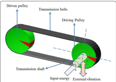
the longitudinal vibration and the transverse vibration. The longitudinal vibration is the vibration along the direction of the center line between the drive pulley and the driven pulley, while the transverse vibration is the vibration in the direction perpendicular to the center line. The transverse vibration is the main cause to the large dynamic stress and fatigue of belts. Therefore, in this section, the dynamic stress is derived considering the comprehensive effects from both the transverse vibration and the longitudinal tension.

To model the transverse vibration of the belts between the drive pulley and the driven pulley, the oxy coordinate sys-tem is established shown in Figure 2. It is assumed that the mass of the belts are uniform with the mass per unit length of and the belts operate with a constant speed of v. The center distance of the pulleys is a. The linear viscous damp-ing coefficient of a belt are represented by γ. The surface load per unit length is denoted by p(x,t) . The tension in the longitudinal direction is presented by u. Then, the motion equation of a single belt span can be expressed as follows:

(1)

ρ

∂2y

∂t2 +g+2v

∂2y ∂x∂t

+

ρv2−u∂

2 y

∂x2 +γ

∂y

∂t +p(x,t)=0.

In general, it is difficult to derive an exact analytic solution of Eq. (1). Therefore, the Galerkin discretiza-tion method [18] and the numerical algorithm are always adopted to acquire an approximate solution. In this paper, the Runge-Kutta method combining the central differ-ence method is used to solve the equation. By consider-ing N1 nodes in the belt span with the distance between two adjacent nodes of Δ, the continuous system is con-verted into a discrete–continuous system and the vibra-tion of the belts in different posivibra-tions can be obtained. The motion equation of the jth node can be given by

where

The displacement and velocity of Node 1 and Node N1 are determined by the boundary condition as follows:

As a matter of fact, the motion of the end points is a significant cause of the dynamic stress on the belts which directly leads to the fatigue failure of belts. In this paper, we assume the motion of the end points follow the functions below:

where e1 and e2 are the amplitudes of Node 1 and Node

N1. w1 and w2 are the angular frequencies of Node 1 and Node N1. φ1 and φ2 are the initial phases of Node 1 and Node N1. For descriptive convenience, denote the above parameters for motion of end points by a vector (2) ¨

yj = −

1 a1

a2yj+1+yj−1+(a3−a2)yj

+pj(t)+a1

g+a4

˙

yj+1− ˙yj−1

,

a1=ρ,

a2=

ρv2−u

�2 ,

a3=γ,

a4= v

.

(3) y(0,t)=f1(t),

(4) ˙

y(0,t)=f2(t),

(5) y(a,t)=_f3(t),

(6) ˙

y(a,t)=f4(t).

(7) f1(t)=e1sin(w1t+φ1),

(8) f2(t)=_e1w1cos(w1t+φ1),

(9) f3(t)=e2sin(w2t+φ2),

(10) f4(t)=e2w2cos(w2t+φ2),

Figure 1 Schematic structure of a belt drive system

Ψ =[e1e2w1w2φ1φ2] . Then, the additional stress on the belts can be further derived as follows:

The total stress on the belts can be expressed by

where A is the cross sectional area of the belts. From the derivation process of σ, it can be seen that Ψ and u

has great influences on dynamic stress on belts. In prac-tice, the randomness of the dynamic stress always comes from u and the amplitudes of f1(t) and f2(t) denoted by Ψ1=[e1e2] . The randomness of u results from the ran-dom initial tension and the ranran-domness of working load, while the randomness of Ψ1 is caused by environmental load including the vibration from other components and the ground vibration. However, owing to the difficulty to derive an explicit solution of Eq. (12), it is impractical to provide an explicit mathematical function to express the relationship between the joint distribution function of Ψ

and u and the distribution function (DF) of σ. Therefore, in this section, the DF of σ is obtained by using the neural network models (NNM).

The NNMs simulate the information processing models of the nervous systems for mathematical simulations [19– 22]. An important element in the NNM is the neuron, whose general schematic structure is shown in Figure 3.

In Figure 3, zi(i = 1, 2, 3,…, n) are the outputs of other neurons which is also the inputs of this neuron. Dif-ferent weight values for the inputs represent difDif-ferent connection strength of the inputs. The relationship between the input variables and the output variables can be expressed as follows:

(11) σ0=

1 2E

∂y ∂x

2

.

(12) σ = 1

2E

∂y ∂x

2

+ u A,

(13) y=F

_n

i=1 wizi

.

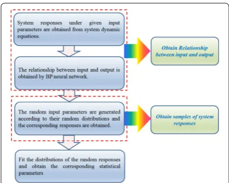
For different neuron models, many NNMs have been proposed, in which back propagation neural networks (BPNN) have been widely used in the field of mechanical engineering [23–26]. The BPNN has many advantages, such as self-learning, self-organization, self-adaptation and the strong ability of nonlinear mapping. A continuous function can be approximated by arbitrary precision via the BPNN. The BPNN is a multilayer feedforward neural network, which consists of input layer, hidden layer and output layer, as shown in Figure 4. The BPNN adopts the whole interconnection mode between adjacent layers, while there is no connection between the same layer. The hidden layer can be composed of one layer or multiple lay-ers. The learning process of BPNN can be summed up as follows.

(1) The input is calculated through the input layer and the hidden layer and outputs from the output layer. In the calculation process, each layer of neurons only affects the next layer of neurons.

(2) If the output layer cannot acquire the desired out-put, it goes to the error back propagation process. The error signal is returned along the original con-nection path, and the weights and thresholds of each layer of the network are adjusted successively until the input layer is reached.

(3) Step 1 and Step 2 are repeated until the desired out-puts are obtained. In this process, the weights and thresholds of each layer are constantly adjusted aiming at achieving the intended design.

Then, the samples of the random response can be obtained by using the above BPNN method with the samples of the random variables of Eq. (1) as the input. The distribution of σ can be gained by fitting the random sample of σ. The whole process is illustrated via the flow-chart shown in Figure 5 as follows.

Figure 3 A schematic neuron model

3 Reliability Models of Belt Drive Systems Considering Failure Dependence

In practice, the drive pulley and the driven pulley seldom failure before the belts. Therefore, in initial operational stage, only the fracture of belts has to be taken into account as the cause of the system failure. However, it should be

In the reliability analysis of belt drive systems, mainte-nance activities or replacements are not taken into account and the failure of the multi-belt systems refers to the first failure of the most vulnerable single belt. Besides, the fail-ure of any belts leads to the system failfail-ure. Thus, the mul-tiple belts logically consist of a series system. Owing to the gradual degradation of the belt strength, the working dura-tion of the multi-belt systems t is discretized to a series of time intervals denoted by ti (i = 1, 2,…, k). Moreover, the remaining strength in each time interval is assumed to be constant, which is expressed as follows:

The remaining strength ri(t) of a single belt in the ith time interval is the function of the initial strength r0 and the stress history σ (t) . The choice of k depends on the descent velocity of the remaining strength.

From Section 2, it can be learnt that all the N belts in a system share the same motion of end points. Besides, the relationship between the maximum stress σj(ti) , Ψ1(ti) and uj(ti) of the jth belt (j = 1, 2,…, N) in the ith time interval is given by

Denote the probability density functions (PDF) of Ψ1(ti) and u(ti) by f(Ψ1(ti)) and.Then, the reliability in the ith time interval can be calculated by

(14)

ri(t)=r(r0,ti,σ (t)), i=1, 2,. . .,k.

(15) σ_j(ti)=f

Ψ1(ti),uj(ti)

.

(16)

R1(ti)=

� ∞

−∞

f(Ψ1(ti))



 N �

j=1

� ∞

−∞

f�

uj(ti)�

× � ∞

f(Ψ1(ti),uj(ti))f �

rij �

rj0,ti,σj(t) ��

drij �

rj0,ti,σj(t) �

duj(ti) 

dΨ1(ti), Figure 5 Flowchart for distribution fitting of system dynamic

responses

noted that the fracture of belts is directly affected by the motion of both the drive pulley and the driven pulley as shown in Eq. (1). Hence, before the maintenance or replacement of the belts and the pulleys, the system reli-ability can be calculated by comparing the dynamic stress

σ on belts and the remaining strength of belts. In conven-tional reliability analysis of belt drive systems in the failure mode of fatigue, a static interference between the static stress on belts and the fatigue limit is always performed by using the SSI model. Nevertheless, from the definition of reliability, it can be known that reliability is a function of time. The static reliability models cannot be used to ana-lyze the dynamic characteristics of the system reliability. Thus, in this section, dynamic reliability models of belt drive systems are developed, which are also the basis for time-dependent availability models of belt drive systems established in the next section.

where rij

rj0,ti,σj(t)

is the remaining strength of the jth belt, which is determined by the initial strength rj0 and the stress history σj(t) of the jth belt. When consider-ing the distributions of the initial strength of the belts, denote the joint PDF of the initial strength of the belts by f(r₀₎ . The reliability of the belt drive systems can be expressed as follows:

(17)

R2(t)= � ∞

−∞

f(r₀) �k

�

i=1

� ∞

−∞

f(Ψ1(ti))

× 



N

�

j=1

�∞

−∞

f�

uj(ti)� �∞

f(Ψ1(ti),uj(ti))

f�

rij�

rj0,ti,σj(t)��

×drij�

rj0,ti,σj(t)�duj(ti)

 dΨ1(ti)

 

In Eq. (17), the failure dependence of the belts in a system is taken into account. Provided that the belts are assumed to be statistically independent with each other, the reliabil-ity is expressed by

where f rj0

is the PDF of the initial strength rj0 of the

jth belt. However, as stated above, all the belts share the same vibration in the driving pulley and that in the driven pulley. Moreover, the stress in each belt is also mutually dependent, which significantly influences the strength degradation dependence of the belts. Therefore, the reliability derived based on conventional independ-ent assumption on the belts does not conform to reality. The corresponding calculation error will be illustrated in the numerical examples. To analyze the impacts of failure dependence on reliability with respect to various param-eters, the dependence sensitivity function (DSF) is pro-posed as follows:

(18) R3(t)=

k

i=1

N

j=1

∞ −∞ f rj0 ∞ −∞ f

Ψj1(ti)

∞

−∞ f

uj(ti)

×

∞

f(Ψj1(ti),uj(ti))

f rij

rj0,ti,σj(t)

×drijrj0,ti,σj(t)

duj(ti)dΨ1(ti)drj0,

(19)

D(t)= ∂[R2(t)−R3(t)]

∂ζ

=∂

�

� ∞

−∞

f(r₀₎

� _k

�

i=1

� ∞

−∞

f(Ψ1(ti))×





N

�

j=1

� ∞

−∞

f�

uj(ti)

�

×

� ∞

f(Ψ1(ti),uj(ti)) f�

rij�rj0,ti,σj(t)��drij�rj0,ti,σj(t)�duj(ti)





×dΨ1(ti)







dr₀−







k

�

i=1 N

�

j=1

� ∞

−∞

f�

rj0�

� ∞

−∞

f�

Ψj1(ti)�

� ∞

−∞

f�

uj(ti)�

×

� ∞

f(Ψj1(ti),uj(ti)) f�

rij

�

rj0,ti,σj(t)

��

drij

�

rj0,ti,σj(t)

�

× duj(ti)dΨ1(ti)drj0

     

/∂ζ,

where ζ is the parameters in system reliability functions, such as the initial strength, motion in end points, tension, etc. In addition, the system failure rate is an important reliability index, which provides guidance for mainte-nance decision making and optimization design. Accord-ing to the definition of failure rate, the failure rate of the belt drive systems can be expressed by

(20)

_1(t)= −dR2(t)

R2(t)dt =d �

� ∞

−∞ f(r₀₎

� _k �

i=1 � ∞

−∞

f(Ψ1(ti))

×   N � j=1 � ∞ −∞ f�

uj(ti) �

� ∞

f(Ψ1(ti),uj(ti))

f� rij

�

rj0,ti,σj(t) ��

×drij�

rj0,ti,σj(t)�duj(ti) 

dΨ1(ti)  

 dr₀

   /       � ∞ −∞ f(r₀)

   k � i=1 � ∞ −∞

f(Ψ1(ti))   N � j=1 � ∞ −∞ f�

uj(ti)�

×

� ∞

f(Ψ1(ti),uj(ti))

f� rij�

rj0,ti,σj(t)��drij�rj0,ti,σj(t)�

× duj(ti)



dΨ1(ti)  

 dr₀

Accordingly, the failure rate of the independent belt drive systems can be given by

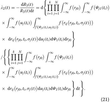
(21)

_2(t)= −dR3(t) R3(t)dt =d







k

�

i=1

N

�

j=1

� ∞

−∞ f�

rj0�

� ∞

−∞ f�

Ψj1(ti)�

×

� ∞

−∞ f�

uj(ti)�

� ∞

f(Ψj1(ti),uj(ti)) f�

rij�rj0,ti,σj(t)��

× drij�rj0,ti,σj(t)�duj(ti)dΨ1(ti)drj0







/ 



 





k

�

i=1

N

�

j=1

� ∞

−∞ f�

rj0�

� ∞

−∞ f�

Ψj1(ti)�

×

� ∞

−∞ f�

uj(ti)�

� ∞

f(Ψj1(ti),uj(ti)) f�

rij�rj0,ti,σj(t)��

× drij�rj0,ti,σj(t)�duj(ti)dΨ1(ti)drj0







dt







.

4 Availability Models of Belt Drive Systems

To guarantee a stable and reliable transmission, multiple belts are used to transfer the load and motion. Moreover, as stated in Section 1, maintenance and replacement of belts are important to maintaining the normal opera-tional state and prolong the lifetime of the belt drive systems. Although the surface adhesion technology for the repair of slightly damage and torn on the protective layers of the belts and the joint repair technology for the repair of severe transverse tear on belts and joint degum-ming have been widely used in the maintenance of belt drive systems, it is difficult for the belts to restore as new products after the maintenance activities. Therefore, the maintenance of the belts is essentially minimal mainte-nance. In this paper, the repair activities are carried out immediately after the failure of any belt and the repair time obeys the exponential distribution.

The repair rate μ is an important maintainability index in availability analysis. In this section, imperfect maintenance is taken into account. To consider the possibility of imperfect maintenance, the repair rate is divided into two categories as follows.

(1) When the belts can be repaired according to the prescribed time with the probability of p, the repair rate is denoted by μ1.

(2) When the belts cannot be repaired within the stipu-lated time with the probability of (1 − p), the repair rate is denoted by μ2, which indicates a longer maintenance duration.

In addition, in the situation where the failure rate of the system is a constant, the calculation of the system availability could be greatly simplified by using the state transition matrix, because the time between two adja-cent failure follows the exponential distribution. How-ever, as mentioned in Section 3, the failure rate of the belt drive systems is time-dependent. Moreover, the index of time t in the failure rate _1(t) and the index of time T in the system availability A(T) are not the same physical quantity, which is explained in Figures 6 and 7. The time t in _1(t) does not include the repair time. The time T in the system availability A(T) includes both the operational duration and the repair time. There-fore, these two different physical quantities should be distinguished in the process of establishing differential Figure 6 Availability with respect to T

equations, which considerably increases the difficul-ties in system availability computation and is seldom reported.

Denote the system availability in the time instant T

and T+T by A(T) and A(T+�T) , respectively. Then, the relationship between A(T) and A(T +�T) can be given by

Then, it can be derived from Eq. (22) that

Denote the first derivative of A(T) by A(T) and Eq. (23) can be rewritten by

The average failure times of the system within t can be calculated as follows:

The corresponding mean maintenance time can be given by

Then, the relationship between t and T can be expressed by

(22)

A(T +�T)=A(T)[1−_1(t)�T]

+(1−A(T))[pµ1�T+(1−p)µ2�T].

(23) A(T+�T)−A(T)

�T =(1−A(T))[pµ1+(1−p)µ2]

−A(T)_1(t).

(24)

A(T)= −[pµ1+(1−p)µ2+1(t)]A(T)

+pµ1+(1−p)µ2.

(25)

N1=

_t

0

_i(τ )dτ.

(26) tm= p

µ1 t

0

_{i(τ )}dτ+ 1−p

µ2 t

0

_{i(τ )}dτ.

Hence, the time-dependent A(T) can be obtained from Eq. (24). It should be noted that the time index of t is not identical with the time index of T in Eq. (24). Hence, Eq. (24) is not an ordinary differential equation (ODE), whose solution needs to be acquired by numerical method. When the difference between t and T is neglected, Eq. (24) becomes an ODE as follows:

The computational error because of this neglect will be demonstrated later. In addition, the availability of the independent systems can be derived by

5 Numerical Examples

Consider a belt drive system consisting of a driving pul-ley, a driven pulley and multiple belts. The material and geometric parameters of the system are shown in Table 1. For descriptive convenience, only the vertical vibration (27) p

µ1

t

0

_i(τ )dτ+ 1

−_p

µ2

t

0

_i(τ )dτ+t=T.

(28)

A1(T)= −[pµ1+(1−p)µ2+1(T)]A1(T)

+pµ1+(1−p)µ2.

(29) A2(T)= −[pµ1+(1−p)µ2+2(t)]A2(T)

+_pµ1+(1−_p)µ2.

Table 1 Geometric parameters and  the  material parameters

Parameter Value

u (N) 150

v (m/s) 5

a (mm) 2000

ρ (kg/m3_{) 1.05 × 10}3

A (mm2_{) 100}

γ (N s/m) 0.3

w₁ (rad/s) 52.3

σlim (MPa) 0.8

C (MPa2_{) 10}19

µ1 (h−1) 30

µ₂ (h−1_{) 50}

m 2

p 0.3

of the driving pulleys is taken into account with e1 fol-lowing the normal distribution. The mean value and the standard deviation of e1, denoted by α(e1) and β(e1) , are 15 mm and 3 mm respectively. The mean value and the standard deviation of r0 are 6 MPa and 1.2 MPa respec-tively. The remaining strength of the jth belt is expressed by [27]

dj is the damage of the ith belt given by

where σ_iq is the stress in the ith time interval that is larger than a specified stress level σlim . Liq is the lifetime under σ_iq in the S–N fatigue curve, which is expressed as follows [28–31]:

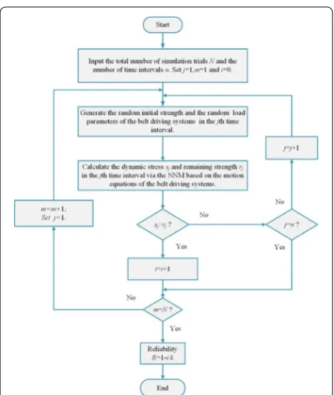
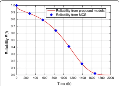
where m and C are material parameters. The Monte Carlo simulation verification is performed with the flow chart shown in Figure 8 and the results shown in Fig-ure 9. Moreover, the reliability and failure rate of the dependent system and those of the independent system are plotted in Figures 10 and 11, respectively. It should be noted that the reliability models and the availability mod-els proposed in this paper take the parameters listed in Table 1 as the inputs, which are not limited by the spe-cific value of these parameters.

From Figures 9, 10 and 11, it can be seen that the pro-posed models can be used for time-dependent reliability assessment of belt drive systems. The results from the proposed models are consistent with the results from the MCS. Besides, the system reliability decreases with time due to the material degradation and the repeated load applications. Correspondingly, the failure rate of the belt drive systems rises with time. Nevertheless, the different assumptions on the dependence of the belts lead to dif-ferent conclusions about the system reliability. In general, the hypothesis that the belts are regarded as independent components indicates a faster decline of reliability. How-ever, the belts share the same load in practice. Hence, the independence assumption about the belts results in an underestimation of reliability despite the computational convenience of reliability models of independent systems. The difference between the reliability of the depend-ent system and the reliability of the independdepend-ent system becomes more obvious with the operation time.

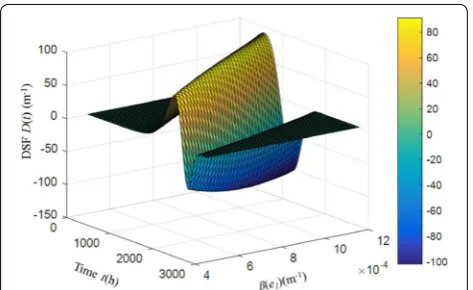
In addition, the DSF curve with respect to the standard deviation of e1 are plotted in Figure 12. From Figure 12, it can be learnt that two peaks appear in the whole

(30) rij =rj01−dj

,

i=1, 2,. . .,k, j=1, 2,. . .,N

.

(31) dj=

k

i=1 q1

q=1 σiq Liq

,

j=1, 2,. . .,k ,

(32)

σ_iqmLiq=C, Figure 9 Reliability from proposed models and reliability from MCS

Figure 10 Reliability of the belt drive system

operation duration, which indicates that there exist two most sensitive moments to the dependence of the belts. In the vicinity of these two moments, particular attention should be paid to the influence of failure dependence on system reliability. Moreover, a backward migration of the

two peaks takes place with the decrease of the standard deviation of e1. The migration of the first peak is more obvious than that of the second peak. Furthermore, the maximum sensitivity also decreases with the decrease of the dispersion of e1.

To analyze the computational error caused by neglect-ing the distinction between t and T, the comparison between the availability A(T) and the availability A1(T) is shown in Figure 1. Besides, the comparison between the availability of the dependent system A(T) and the availability of the independent system A2(T) is shown in Figure 13. Finally, the time-dependent system availabili-ties under different value of p rather than a constant of 0.3 are shown in Figure 14.

From Figure 13 it can be learnt that the system avail-ability decreases with time. Similar to the system reli-ability, the failure dependence of the belts causes a promotion of system reliability. The independence assumption about the belts leads to an underestimation of the availability of the belt drive systems. In addition, the time scale of the failure rate and the time scale of the availability are inconsistent. The neglect of the time scale inconsistency could underestimate the system avail-ability. Therefore, when the failure rate data of the belt drive systems is adopted in the availability analysis, atten-tion should be paid to this time scale inconsistency. Fur-thermore, from Figure 14 it can be learnt that imperfect maintenance is taken into consideration in the proposed models. With the increase of the probability of imperfect maintenance, the system availability declines faster. The effects of imperfect maintenance on system availability become more obvious with time.

6 Conclusions

Conventional reliability models of belt drive systems in the failure mode of fatigue are mainly based on the static SSI model and its extended models. The dynamic stress on the belts and the degradation of material properties of belts cannot be considered in these mod-els. Moreover, a time-dependent availability analysis of belt drive systems cannot be performed based on a static reliability index. To include these dynamic factors in the reliability analysis of belt drive systems and carry out a further system availability analysis, time-depend-ent reliability models, failure rate models and availabil-ity models of belt drive systems are developed in this paper. MCSs are used to validate the established els. In the reliability models and the availability mod-els, dynamic failure dependence is taken into account, which has significant influences on system reliability and system availability. These influences show obvious time-dependent characteristics. In addition, the issue of time scale inconsistency between system failure rate Figure 12 DSF curve of the belt drive system

Figure 13 Availability of the belt drive system

and system availability is proposed in this paper and considered in the proposed system availability models. The results show that the effects of time scale incon-sistency on system availability are time-dependent and remarkable. Therefore, in practice, special attention should be paid to the usage of the collected failure rate data for system availability analysis due to the existence of the time scale inconsistency.

Authors’ Contributions

PG and LX contributed the central idea, analyzed most of the data, and wrote the initial draft of the paper. JP contributed to refining the ideas, carrying out additional analyses and interpreting the results. All authors read and approved the final manuscript.

Author Details

1 _{School of Mechanical Engineering, Liaoning Shihua University,} Fus-hun 113001, China. 2 _{School of Mechanical Engineering and Automation,} Zhejiang Sci-Tech University, Hangzhou 310018, China. 3 _{School of Mechanical} Engineering and Automation, Northeastern University, Shenyang 110819, China.

Authors’ Information

Peng Gao, born in 1982, is currently an associate professor at Liaoning Shihua University, China. His main research interests include system reliability analysis and dynamics of machinery.

Liyang Xie, born in 1962, is currently a professor and a PhD candidate supervisor at Northeastern University, China. His main research interests include system reliability and structural fatigue.

Jun Pan, born in 1974, is currently a professor at Zhejiang Sci-Tech Uni-versity, China. His main research interests include reliability engineering and accelerated life test.

Competing Interests

The authors declare that they have no competing interests.

Funding

Supported by Program for Liaoning Innovative Talents in University (Grant No. LR2017070), National Natural Science Foundation of China (Grant No. 51505207), Open Foundation of Zhejiang Provincial Top Key Academic Discipline of Mechanical Engineering (Grant No. ZSTUME02A01), and National Natural Science Foundation of China (Grant No. U1708255).

Received: 29 November 2017 Accepted: 12 March 2019

References

[1] N Nevaranta, J Parkkinen, T Lindh, et al. Online estimation of linear tooth belt drive system parameters. IEEE Transactions on Industrial Electronics, 2015, 62(11): 7214–7223.

[2] B Balta, F O Sonmez, A Cengiz. Experimental identification of the torque losses in V-ribbed belt drives using the response surface method. Proceedings of the Institution of Mechanical Engineers Part D Journal of Automobile Engineering, 2015, 229(8): 1070–1082.

[3] B Balta, F O Sonmez, A Cengiz. Speed losses in V-ribbed belt drives. Mechanism and Machine Theory, 2015, 86(86): 1–14.

[4] S Abrate. Vibrations of belts and belt drives. Mechanism & Machine Theory, 1992, 27(6): 645–659.

[5] Z W An, H Z Huang, D Lin. An approach to reliability evaluation of multi-ple V-belt drives considering the deviation of belt length. Proceedings of the Institution of Mechanical Engineers Part O Journal of Risk and Reliability, 2009, 223(2): 159–166.

[6] X P Bai, J J Mu. Research on three-parameter weibull distribution in failure data processing and dynamic reliability evaluating of belt transportation

system in mines. Journal of NanjingUniversity ofScienceand Technology, 2011, 35(2): 97–101.

[7] X P Gong, C L Tong, W J Liu. Research on reliability-based optimum design procedure for type -V belt transmission. Journal of Air Force Engi-neering University, 2002, 3(4): 65–68.

[8] C Sun, A Ren, G Sun, et al. The calculation of the classical V-belt life with different reliability. Procedia Engineering, 2011, 15(1): 5290–5293. [9] D Mazurkiewicz. Computer-aided maintenance and reliability

manage-ment systems for conveyor belts. Eksploatacja i Niezawodnosc - Mainte-nance and Reliability, 2014, 16(3): 377–382.

[10] Y Sahraoui, R Khelif, A Chateauneuf. Maintenance planning under imper-fect inspections of corroded pipelines. International Journal of Pressure Vessels and Piping, 2013, 104(1): 76–82.

[11] P Dehghanian, M Fotuhifiruzabad, F Aminifar, et al. A comprehensive scheme for reliability centered maintenance in power distribution systems—Part I: Methodology. IEEE Transactions on Power Delivery, 2013, 28(2): 771–778.

[12] S K Abeygunawardane, P Jirutitijaroen, H Xu. Adaptive maintenance poli-cies for aging devices using a Markov decision process. IEEE Transactions on Power Systems, 2013, 28(3): 3194–3203.

[13] T B Kumar, O C Sekhar, M Ramamoorty, et al. Evaluation of power capac-ity availabilcapac-ity at load bus in a composite power system. IEEE Journal of Emerging & Selected Topics in Power Electronics, 2016, 4(4): 1324–1331. [14] Y Lee. Availability analysis of redundancy model with generally

distrib-uted repair time, imperfect switchover, and interrupted repair. Electronics Letters, 2016, 52(22): 1851–1853.

[15] N Jack. Age-reduction models for imperfect maintenance. IMA Journal of Management Mathematics, 2018, 9(4): 347–354.

[16] H Ding, J W Zu. Effect of one-way clutch on the nonlinear vibration of belt-drive systems with a continuous belt model. Journal of Sound and Vibration, 2013, 332(24): 6472–6487.

[17] H Ding, D P Li. Static and dynamic behaviors of belt-drive dynamic sys-tems with a one-way clutch. Nonlinear Dynamics, 2014, 78(2): 1553–1575. [18] F Zhu, R G Parker. Piece-wise linear dynamic analysis of serpentine belt

drives with a one-way clutch. Proceedings of the Institution of Mechanical Engineers Part C Journal of Mechanical Engineering Science, 2008, 222(7): 1165–1176.

[19] Z Boger, H Guterman. Knowledge extraction from artificial neural network models. Journal of Renewable and Sustainable Energy, 2015, 4(5): 3030–3035.

[20] H M R Ugalde, J C Carmona, Reyes-Reyes J, et al. Computational cost improvement of neural network models in black box nonlinear system identification. Neurocomputing, 2015, 166(C): 96–108.

[21] K Benmouiza, A Cheknane. Small-scale solar radiation forecasting using ARMA and nonlinear autoregressive neural network models. Theoretical and Applied Climatology, 2016, 124(3-4): 945–958.

[22] M Gevrey, I Dimopoulos, S Lek. Review and comparison of methods to study the contribution of variables in artificial neural network models. Ecological Modelling, 2003, 160(3): 249–264.

[23] R Huang, L Xi, X Li, et al. Residual life predictions for ball bearings based on self-organizing map and back propagation neural network methods. Mechanical Systems and Signal Processing, 2007, 21(1): 193–207. [24] R R Srikant, P V Krishna, N D Rao. Online tool wear prediction in wet

machining using modified back propagation neural network. Proceed-ings of the Institution of Mechanical Engineers Part B Journal of Engineering Manufacture, 2011, 225(7): 1009–1018.

[25] J Zhang, C Xu, M Yi, et al. Design of nano-micro-composite ceramic tool and die material with back propagation neural network and genetic algorithm. Journal of Materials Engineering and Performance, 2012, 21(4): 463–470.

[26] A T Hammid, M H B Sulaiman, O I Awad. A robust firefly algorithm with backpropagation neural networks for solving hydrogeneration predic-tion. Electrical Engineering, 2018, 100(4): 2617–2633.

[27] Y W Gu, W G An, H An. Structural reliability analysis under dead load and fatigue load. Acta Armamentari, 2007, 28(12): 1473–1477.

[29] L Davide, J Maljaars, H H Snijder. Fitting fatigue test data with a novel S-N curve using frequentist and Bayesian inference. International Journal of Fatigue, 2017, 105(12): 28–143.

[30] S Hou, J Xu. An approach to correlate fatigue crack growth rate with S-N curve for an Aluminum alloy LY12CZ. Theoretical and Applied Fracture Mechanics, 2018, 95(6): 177–185.