R E S E A R C H A R T I C L E
Open Access
Estimation of error in observables of
coarse-grained models of atomic systems
John Tinsley Oden
*, Kathryn Farrell and Danial Faghihi
*Correspondence: [email protected] Institute for Computational Engineering and Sciences The University of Texas at Austin, 201 East 24th St, Stop C0200 POB 4.102, 78712 Austin, TX, USA
Abstract
Background: The use of coarse-grained approximations of atomic systems is the most common methods of constructing reduced-order models in computational science. However, the issue of central importance in developing these models is the accuracy with which they approximate key features of the atomistic system. Many methods have been proposed to calibrate coarse-grained models so that they qualitatively mimic the atomic systems, but these are often based on heuristic arguments.
Methods: A general framework for deriving aposterioriestimates of modeling error in coarse–grained models of key observables in atomistic systems is presented. Such estimates provide a new tool for model validation analysis. The connection of error estimates with relative information entropy of observables and model predictions is explained for so-called misspecified models. The relationship between model
plausibilities and Kullback-Leibler divergence between the true parameters and model predictions is summed up in several theorems.
Results: Numerical examples are presented in this paper involving a family of coarse-grained models of a polyethylene chain of united atom monomers. Numerical results suggest that the proposed methods of error estimation can be very good indications of the error inherent in coarse-grained models of observables in the atomistic systems. Also, new theorems relating the Kullback-Leibler divergence between model predictions and observations to measures of model plausibility are presented. Conclusions: A formal structure for estimating errors produced by coarse-graining atomistic models is presented. Numerical examples confirm that the estimates are in agreement with exact errors for a simple class of materials. Errors measured in the DKL-divergence can be related to computable model plausibilities. The results should provide a powerful framework for assessing the validity and accuracy of coarse-grained models.
Keywords: Molecular dynamics, Coarse–grained models, Adjoint systems, Information entropy
Background
Coarse-grained-reduced order models
The most common method of constructing reduced-order models in all of computational science involves the use of coarse-grained models of atomic systems, whereby systems of atoms are aggregated into “beads”, or “super atoms”, or molecules to reduce the number of degrees of freedom and to lengthen the time scales in which the evolution of events are simulated.
The use of coarse-grained (CG) approximations has been prevalent in molecular dynamics (MD) simulations for many decades Comprehensive reviews of a large segment of the literature on CG models was recently given by Noid [1] and Liet al.[2], and an application to semiconductor nano-manufacturing is discussed in Farrellet al.[3]. The issue of central importance in developing CG models is the accuracy with which they approximate key features of the atomistic system. Many methods have been proposed to calibrate CG models so that they qualitatively mimic the all-atom (AA) systems, but these are often based on heuristic arguments.
In this paper, we develop a posteriori estimates of error in CG approximations of
observables in the AA system. We focus on standard molecular dynamics models of micro-canonical ensemble (NVE) thermodynamics, and we call upon the theory of model adaptivity and error estimation laid down in [4] and [5]. In this particular setting, new esti-mates are also obtained when the information entropy of Shannon [6] is used as a quantity of interest. This leads to methods for estimating CG-model parameters that involve the Kullback-Leibler divergence between probability densities of observables in the AA and CG systems.
In the finalResults and discussionsection of this presentation, we review several sta-tistical properties of parametric models, including asymptotic properties of misspecified models and generalizations of the Bernstein-von Mises theorem advanced by Kleijn and van der Vaart [7]. There, the fundamental role of the Kullback-Leibler distance (theDKL) between the true probability distribution and the observations accessible by the model is reviewed. We present results in the form of theorems that relate theDKLto measures of model plausibility that arise from Bayesian approaches to model selection. The rela-tionships of thea posterioriestimates to the statistical interpretations are summarized in concluding remarks.
Preliminaries, conventions and notations
We generally approach the problem of developing computer models of large atomic sys-tems through the use of any of several hardened molecular dynamics (MD) codes or through equivalent Monte Carlo approximations invoking the ergodic hypothesis. For a system ofnatoms, the Hamiltonian is
Hrn,pn=
n
α=1 mα
2 pα·pα+u(r
n), (1)
wherern= {r1,r2,. . .,rn}is the set of atomic coordinate vectors,pn= {p1,p2,. . .,pn}is the set of particle momentum vectors,mαthe atomic mass of theα−th atom andu(rn)is the potential energy or interaction potential. Then(rn,pn)defines a point or microstate in the phase spaceAAof the all atom (AA) model. In typical MD simulations, the potential is, for example, of the form
u(rn)=Vbond(rn)+Vangle(rn)+Vdihedral(rn)+Vnon-bonded(rn)+Vcoulomb(rn), (2)
where
Vbond(rn)= Nb
i=1 1
2kri|ri−r0i|
Vangle(rn)= Na
i=1 1
2kθi(θi−θ0i)
2, (3b)
Vdihedral(rn)= Nnb−1
i=1 Nnb
j=1 Vji
2
1+(−1)j−1cos(jφi)
, (3c)
Vnon-bonded(rn)= Nnb
i=1
j>i 4ij
σ
ij rij
α
−
σ
ij rij
β
, rij≤r2, (3d)
Vcolumb(rn)= Nq−1
i=1 Nq
j>i 40
qiqj rij
. (3e)
Here covalent bonds are represented by the harmonic potential (1a), changes in bond angles by (1b), torsional potentials by changes in dihedral angles (1c), Lennard-Jones non-bonded potentials by (1d), withrij = |ri−rj|andrcthe cut-off radius,(α,β)typically =(12, 6), and Coulomb potentials between chargesqiatriandqjatrj(1e). These forms are typical of those implemented in popular MD codes, although several other common potentials could be added. The parameters of the potential model are given by the vec-tor of physical coefficients:{ki,kθi,Vji,φi,ij,σij,rc,. . .}. In general, atomic properties and values of parameters for the full all-atom system are supplied by systems calibrated using experimental data or quantum mechanics predictions (see, e.g. the OPLS data in [8,9]).
Given the Hamiltonian (1), Hamilton’s equations of motion are:
∂H
∂pα = ˙rα,
∂H
∂rα = −˙pα, 1≤α≤n. (4)
In MD, it is assumed that the atomic system evolves according to the laws of Newtonian mechanics, so we setpα =m(α)r˙α, and the second Hamiltonian equation in (4) reduces to the system of equations
mαβ¨rβi(t)+∂αiu(rn(t))−fαi(t)=0, 1≤α,β≤n, 1≤i≤3, (5)
where repeated indices are summed throughout their range,mαβ =m(α)δαβis the mass of atomα, superimposed dots indicate time derivations,rβi is the component ofrβ in
directioni,∂αi=∂/∂rαiu(rn(t))is the total interatomic potential of the system given, e.g., by (2), andfαi(t)is theith component of applied force on atomαat timet. We will add initial conditions,r˙βi(0) =vβi, andrβi(0) =rβ0i, wherevβiandr0βi, for now, are assumed to be given.
Molecular dynamical equations of the form (5) are typical of those in standard MD codes that are numerically integrated with randomly-sampled initial conditions over time intervals to approximate systems with constant energy and fixed volume and fixed num-ber of particles corresponding to so-called micro-canonical ensembles. Without loss in generality, we confine this development to such thermodynamic scenarios noting that straightforward extensions to, say, constant temperature settings, are covered by replacing (5) with appropriate “thermostat” models, such as the Langevin or Nose–Hoover formu-lations (see e.g. [10]). The general approach is then applicable to canonical ensembles and more general statistical thermodynamics settings.
averages over a time intervalτ of some phase function q(rn,pn) that depends on the phase-point positions(rn,pn)in phase space AA, as all measurements require a finite duration. Moreover, for thermodynamic systems in equilibrium, this average, denotedq, must be independent of the starting timet0and it must attain a value from an essentially infinite time duration. Thus, our goal in constructing the all-atom model is to compute observables of the form (cf [10,11]),
q = lim
τ→∞τ −1
t0+τ t0
q(rn(t),pn(t))dt. (6)
Here we shall confine our attention to phase functions that depend only on the con-figurations of systems in thermodynamic equilibrium. Ourquantities of interestare then written,
Qr= lim τ→∞τ
−1 t0+τ
t0
q(rn(t))dt. (7)
In all but the simplest applications, it is impossible to solve the dynamic system (5) owing to its enormous size. Therefore, reduced-order models must be developed. The process involves aggregating groups of atoms into beads or molecules or “super atoms” so as to create a coarse-grained (CG) molecular model. The CG model hasNcoordinate vectorsRN(t) = {R1(t),R2(t),. . .,RN(t)}, N < n; and the corresponding equations of motion are
MABR¨Bi(t)+∂AiU(RN(t),θ)−FAi(t)=0, 1≤A,B≤N, 1≤i≤3. (8)
MABdefining the CG mass matrix,∂Ai=∂/∂RAi,U(·,·)the interaction potential energy of the CG system,θ a vector of parameters defining the CG model, andFAi(t)the ith component of applied force at beadAat timet. Initial conditions areR˙Ai(0) = VAi, and RAi(0)=R0Ai. The unknown parameters with a potential of the form (2) are denoted, for example,
θ =(KRi,R0i,Kθi,θ0i,V0i,εii,σii,· · ·), (9)
the notation, in analogy with (1), being chosen to indicate parameters of the CG model. It is important to establish a kinematic and algebraic relation between coordinates of particles in the AA system and those in the CG system. A very large literature exists on various coarse-graining mapping schemes, and choices of the appropriate map from the AA to the CG system or vice versa are often based on heuristic methods (see e.g. [2]). Our general approach can be adapted to any such well-defined AA-to-CG or CG-to-AA map, but for definiteness, we describe one such family of mappings.
Let JA be the index set of AA-coordinate labels of atoms aggregated into a single
beadAwith CG-coordinate vectorRA emanating from the origin to a reference point
labeledAwithin the bead (e.g.RAcould be chosen to define the center of mass,RA =
α∈JAmαrα/MA,MA=
α∈JAmα). LetaAα(t)be a vector from the reference center of beadAto the end point of AA-coordinate vectorrα(t),α∈JA. LetG·αAbe component of
then×Narray,
G·αA=
1 if α∈JA
Then we have,
rα =
N
A=1
G·αA(RA+aAα), 1≤α≤n. (11)
Here we assume that each AA coordinate vectorrαbelongs to only one bead identified with CG vectorRA, but this is not a necessary assumption. In the case of bonded systems in whichrα is associated with, say, two index setsJAandJB, we simply choose either
JAorJBas the representative ofrαand associaterαwith only one bead to avoid double counting.
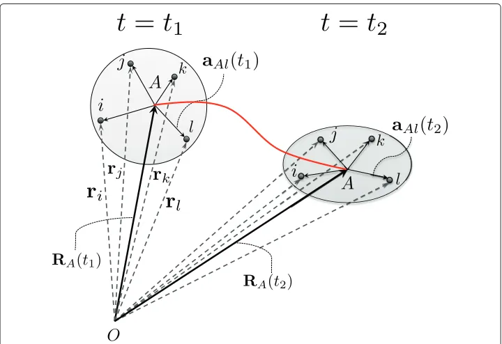
These kinematical conventions are illustrated in Figure 1. The AA coordinatesrα of
atoms assigned to molecular bead A remain with that bead throughout all possible
motions of the CG system. The Boolean arrayG·αAmerely adjusts labels of the AA system to agree with labels assigned beads in the CG system.
Returning to (7), it is clear that the CG approximation of the quantities of interest (QoI) are of the form,
QR(θ)= lim τ→∞τ
−1 t0+τ
t0
qGRN(t),θdt (12)
where G is the AA-to-CG map defined in (11), where we denote rn = G(RN(t),θ), and where we specifically present the dependence of the QoI on the CG potential parametersθ.
Now it is obvious that the evolution of the CG system defined by the coordinate vectors
RA(t)satisfying (8) do not satisfy the “true” equations of motion (5). Indeed, ifRN(t)= {R1(t),R2(t),. . .,RN(t)}is the set ofN-vectors satisfying (8), they constrain the motion
Figure 1 A Lagrangian description of the motion of a molecular beadAand its associated AA atoms
of the AA system via (11), so upon introducing the constrained motions into (5) we obtain the residual,
ραi(θ,t) = mαβ
N
A=1
G·βAR¨Ai+ ¨aAβi(t)
+∂αiu
G(RN(t),aN(t))− N
A=1
G·βAωαβFAi(t),
1≤α,β≤n, 1≤i≤3, (13)
whereβωβα =1,α∈J
Afα=FA, and
G(RN(t),aN(t)) =
A
G·1A(RA+aA1),G·2A(RA+aA2)
. . .,G·nA(RA+aAn)
,
= rn(t). (14)
On the left-hand side of (13), we have taken note that the residual depends on the CG-model parametersθ, not explicitly presented on the right for simplicity. The AA forcefα
at coordinateα is a fractionωαβ of the CG forceFAi. In general, as a first-order approxi-mation, one can take the vectorsaAαas time-independent constant vectors equal to their value in a given reference configuration(aAα(t) = aAα(t0);a˙Aα = ¨aAα = 0). Then the approximate residual results of the form
ˆ
ραi(θ,t)=Gα·AmαβR¨Ai+∂αiuG(RN(t)),aN(t0)−fαi, (15) withfαi=ωβαG·βAFAi, and with repeated indices summed, 1≤α,β≤n, 1≤A≤N.
It is possible to define a reverse or “push back” relationship that assigns to every AA coordinate vectorrαthe CG coordinate vectorRAof the bead to whichrαbelongs. Given
rα, set
RA=G·Aα(rα−aAα), 1≤A≤N, (16)
whereG·Aαis the transpose ofG·αA(no sum onα).
Thus, for each time t ∈[t0,τ], one can select a sample ω(t) of AA coordinates {r∗1(t),r∗2(t),. . .,r∗n(t)} and employ (16) to generate the corresponding CG coordinates {R∗1(t),R∗2(t),. . .,R∗N(t)}. We use the simplified notation,
RN(t)=G(ω(t)) (17)
to define the image of this sample in the CG system.
Methods
Weak forms of the dynamical problem
It is convenient to recast the molecular dynamics problem into a weak or variational form. Toward this end, we introduce the Banach spaces
V=
rn(t);rα∈⊂R3×H2(0,τ); 1≤α≤n;
rn(·)2=
τ
0
[r¨α· ¨rα+ ˙rα· ˙rα+rα·rα] dτ <∞
,
and the semilinear and linear formsB:V×V→R,F:V→R, given by
Brn;vn=
τ
0
mαβ¨rα(t)·vβ(t)+ ∂αiu
rn(t)vαi(t)
dt+I0(vn), (19)
Fvn=
τ
0
fαi(t)vαi(t)dt+vαi(0)mαβVβ− ˙vαi(0)mαβr0β, (20)
where
I0(vn)=vαi(0)mαβ˙rβ(0)− ˙vαi(0)mαβrβ(0). (21)
The notationB(·;·)is intended to mean thatB(·;·)is possibly nonlinear in entries to the left of the semi-colon and linear in the entries to the right of it.
The problem of findingrn∈Vsuch that
Brn;vn=Fvn ∀vn∈V, (22)
is equivalent to (8) in the sense that every solution of (8) with appropriate initial conditions, satisfies (22), and any sufficiantly smooth solution of (22) satisfies (8).
The adjoint problem Let
B(rn;zn,vn)= lim
θ→0θ
−1B(rn+θzn;vn)−B(rn;vn) (23) and
Q(rn;vn)= lim
θ→0θ
−1Q(rn+θvn)−Q(rn), (24) whereQis a functional onV, and bothB(·;·)andQ(·;·)are assumed to exist and be finite (i.e.B(·;·)andQ(·)are Gateaux differentiable). Then the adjoint or dual problem associated with (22) is
Findzn= {z1,z2,. . .,zn} ∈Vsuch that
B(rn;zn,vn)=Q(rn;vn) ∀vn∈V. (25) Introducing (19) into (23) gives, after some manipulations,
B(rn;zn,vn) =
τ
0
mαβz¨βi−Hαiβj(rn(t))zβj
vαidt
+ ˙mαβzβi(τ)vαi(τ)
−mαβz˙βi(τ)vαi(τ), (26)
whereHαiβjis the Hessian,
Hαiβj(rn(t))= ∂
2u(rn(t))
∂rαi∂rβj
. 1≤α,β ≤n, 1≤i,j≤3. (27)
Likewise, ifQ(rn)=0τq(rn(t))dt, then
Q(rn(t);vn)=
τ
0 ∂αi
q(rn(t))vαidt. (28)
Note that (25) is solved “backward in time;” the forward problem (22) is solved forrn(t), which determines the coefficients in B(rn;zn,vn) which marches the adjoint solution fromt=τ tot=0. The dynamical system corresponding to (25) is:
mαβ¨zβi+Hαiβj
rn(t)zβj(t)=∂αiq
Theory of a posteriori estimation of modeling error
Let us now review the theory ofa posterioriestimation of modeling error advanced in [4] and expanded in [5]. We consider an abstract variational problem of finding an elementu in a topological vector spaceVsuch that,
B(u;v)=F(v), ∀v∈V, (30)
whereB(·;·)is a semilinear form fromV×VintoRandF is a linear functional onV. Problem (30) is equivalent to the problem of finding a solutionuof the problemA(u)=F in the dual spaceV, whereAis the map induced byB(·;·):A(u),v =B(u;v)=F(v)= F,v,·;·denoting duality pairing inV×V. Assuming (30) is solvable foru, we wish to compute the valueQ(u)of a functionalQ:V→Rrepresenting a quantity of interest, or an observable of interest.
We assume that the semilinear formB(·;·)and the functionalQ(·;·) are three times Gateaux differentiable onV with respect to u. In particular, the following limits exist (recall (23) and (24)),
B(u;w,v) = lim
θ→0 θ−1[B(u+θw,v)−B(u,v)] Q(u;v) = limθ→0 θ−1[Q(u+θv)−Q(u)]
. (31)
with similar definitions of higher-order derivatives, e.g. B(u;w1,w2,v), B(u;w1,w2, w3,v),Q(u;w,v),Q(u;v1,v2,v3), etc. See [5] for details.
The adjoint problem associated with (30) and the quantity of interest Qconsists of findingz∈Vsuch that
B(u;z,v)=Q(u;v), ∀v∈V. (32)
Now let u0 be an arbitrary element selected in V. The residual functional (or
“residuum”) associated withu0is defined as the semilinear functionalR:V×V →R,
R(u0;v)=F(v)−B(u0;v), (33)
which, for eachu0∈V, is a linear functional onV.
Obviously, ifu0=u, the solution of (30),R(u;v)=0 ∀v∈V. Thus,R(u0;v)describes the degree to which the vectoru0fails to satisfy the central problem (30).
We now recall the basic theorem in [5]:
Theorem 1. Let the semilinear formB(·;·)in (30) and the quantity of interest Q be three-times continuously Gateaux differentiable onV. Let u0be an arbitrary element ofV. Then the error in Q(u)produced by replacing u by u0is given by:
Q(u)−Q(u0)=R(u0;z)+ (34)
whereis a remainder involving higher-order terms in e0 = u−u0andε0 =z−z0, z0 being an approximation of z.
An explicit form ofis given in the appendix.
Ifu0is not an arbitrary vector taken fromV but is a solution of a surrogate problem approximating (30) (such as a coarse-grained model approximating an AA model), then it often happens thatis negligible compared to the residual. Then (34) reduces to the approximation,
This relation is the basis for many successful methods ofa posteriorierror estimation of both modeling error and numerical error. WheneverB(·;·)is a bilinear form andQ(·) is linear,≡0.
A–posteriori estimation of error in CG approximations
The CG approximations of the “ground truth” AA system are characterized by a paramet-ric classP(θ)of molecular dynamics models, one model corresponding to each choice
of the vectorθ in a space of parameters defining the CG intermolecular potential
U(RN(t),θ). For a given value ofθ, observables of interest in states of thermodynamic equilibrium of the CG system are typically generated as averages of samples of the observ-ables taken over subintervals [tk,tk+1]⊂[ 0,τ], for a distribution of initial conditions (see, e.g. [10]).
If we employ the approximation (35) to the AA and CG models, then an estimate of the error in CG approximations of the observable is immediate. Letq(rn)be a phase function whose ensemble averageqis an observable of interest, denotedQras in (7). The CG
approximation isQR(θ)and the error, given by (35), is
ε(θ)=Qr−QR(θ)≈R(RN(θ);zn), (36)
whereR(RN(θ);zn) = 0τραi(θ,t)zαi(t)dt,ραi(θ,t)is the residual in (13) (or (15)), and
znis the solution to the corresponding adjoint problem, and is generally unknown. IfZn
is an approximation ofzn, then
|ε(θ)| ≤ |R(RN(θ);Zn)| +C(θ)zn−Zn (37)
with
C(θ)= sup
vn∈V
R(RN(θ,t))V vn
V (38)
· Vbeing the norm on the dual spaceV. The problem of error estimation thus reduces to one of developing efficient procedures to compute the residual (ρ) and to compute reasonable approximations ofzn.
It is clear that a quantitative estimate such as (36) (or an approximation withznreplaced byZn) could be a powerful tool for determining validity of the CG model or in designing validation experiments for CG models. In theory, it also provides a basis for selecting optimal parameters for a given model so as to manageε(θ). We elaborate on this notion in the final part of theResults and discussionsection.
Results and discussion
lengthl, the initial velocities are zero, and the system is assigned an initial displacement fieldui(0)=f(ri), wheref(ri)=1.2e−0.1ri(0). Under these conditions, the AA system (5) reduces to
mu¨−ku=0, u(0)=u0, u˙(0)=v0, (39)
wheremandk are the mass matrix and the stiffness matrix of the united atom system and are of the form
m=m ⎡ ⎢ ⎢ ⎣ 1
. .. 1
⎤ ⎥ ⎥
⎦, k=k
⎡ ⎢ ⎢ ⎢ ⎢ ⎢ ⎢ ⎣
2 −1
−1 2 . .. . .. ... −1 . .. −1 2
⎤ ⎥ ⎥ ⎥ ⎥ ⎥ ⎥ ⎦
. (40)
A familyMof CG approximations of this model is obtained by aggregating the atoms
into beads, with CG models inMdistinguished by the numberPof atoms per CG bead.
The resulting CG system (8) is of the form
MU¨ −K U=0, U(0)=U0, U˙(0)=V0, (41)
with the mass of each bead set toM=Pmand the bond stiffnessK=αk/P;α∈R+. Upon solving (41) for the CG displacement trajectoryU(t), we compute the residual trajectory
ρ=mU¨CG−kUCG, (42)
whereUCG(t)is the projectionU(t)onto AA atom locations.
The bilinear and linear forms described in (19)-(21) reduce, in this case, to
B(u;v) =
τ
0
vT(mu¨−ku)dt−vT(0)mu˙(0)− ˙vT(0)mu(0), (43)
F(v) = −vT(0)mv0− ˙vT(0)mu0. (44)
and (25) yielding
B(u;v,z) = τ
0 (
mz¨−kz)Tvdt (45)
+ (mz(τ))Tv˙(τ)−(m˙z(τ))Tv(τ) = Q(v).
As an example of a QoI, we takeQrto be the locally-averaged displacement,
Qr=
τ
0 ζ(
t)dt; ζ(t)= 1 N0
i∈N
ui(t); N = {i:xi≤βl;β∈R+}, N0=cardN, (46)
for which the strong form of the dual problem is
m¨z−kz=q, mz˙(τ)=0, z(τ)=0, (47)
whereN0is the number of united atoms considered in setN andqis the vector defined such thatQ(u)=qTu. Given the QoI (46),qwill be as an×1 vector,
qi= ⎧ ⎨ ⎩
1 ifxi≤βl
0 otherwise
The residual functionR(·,·)of (36) in this example is of the form
R(UCG,zn)=
τ
0 ηt(
t)dt; ηt(t)= n
i=1
zi(t)·ρi(t)dt. (49)
The estimated error in the QoI is then
Eest.=R(UCG,zn)≈Qr−QR, (50)
whereQR =
τ
0 ηt(t)dtand then the exact error is
Eexact=Eest.+, (51)
being the remainder in (34). Since the forms in (43)-(46) are linear in their respec-tive arguments, the exact remaindershould be zero, but the error introduced by the numerical integration schemes employed generally leads to an additional numerical error
t=0. We employ a converted Runga-Kutta algorithm here to integrate (39), (41), and (47).
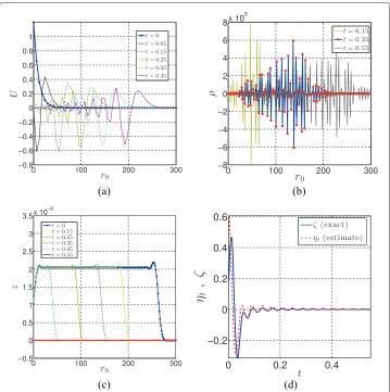
The results of the coarse-grained model for the case ofP=4 are presented in Figure 2. Figure 2a shows the coarse-scale displacementU = U(t)at different times, obtained from solution of (41) over the time domain t ∈[ 0,τ]. The local residual of Figure 2b is then computed from (42). Figure 2c shows the solution of z(t) at different times. It observed that the adjoint solution propagates in time in the opposite direction to the primal solution, (47) being integrated backward in time.
It is known that in general, the solution of the base model is not available. However, in order to show the effectiveness of the method presented here, the equations of motion for the united atom system is also solved in this example. Having the solution of the united atom model,u(t), the evolution of the exactζ and estimatedηt over time is shown in Figure 2d.
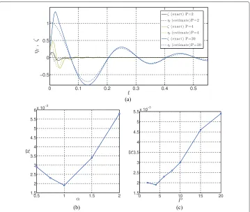
Numerical approximations to the exact error are compared with the estimated error for various CG approximation of the united atom model in Figure 3a. The estimated error
R=R(UCG(θ);zn)for various values ofP, withθ =αk/P, are indicated in Figure 3b for
α=1. The computed estimated error (Eest=R) versus the parameterαare indicated in Figure 3c.
In general, the solution of the base model is not available, but the effectiveness of the method presented here is determined by comparing the CG solutions with the exact united atom model. The exactζ and estimatedηtover time are shown in Figure (2d).
Maximum entropy principle for atomic systems
Among features of the AA system that could qualify as quantities of interest, we consider a special measure of uncertainty content embodied in the so-called information entropy. In 1948, Shannon [6] introduced the concept of information entropy as a real-valued functionH(p)of probability distributions (densities)pas a logical measure of uncertainty content inpthat satisfied four rather straight forward “common-sense” desiderata (see also [12] for full details). For a discrete pdfp= {p1,p2,. . .,pn}, the entropy is defined by
H(p)= − n
i=1
Figure 2 Numerical solutions of the coarse-grained model. Coarse-grained model of a polyethylene chain containing 200 monomers with 4 united atoms per coarse-grained bead,P=4,α=1, andβ=4:(a) coarse-scale displacement,U(t);(b)local residualρ(t);(c)adjoint solution,z(t);(d)time evolution in estimated and exact error in QoI,ηt.
and for a continuous density,p∈L2(R), we write
H(p)= −
Rp(y)logp(y)dy. (53)
Given two probability densities p and q, with non-empty support of domains, the
relative entropy betweenpandqis given by the Kullback-Leibler divergence,
DKL(pq) =
Rp(y)log p(y) q(y)dy
= H(p,q)−H(p), (54)
whereH(p,q)(= −Rplogqdy) is the cross entropy and it is understood that 0 log00=0 and 0 log0q=0.
Shannon’s principle of maximum entropy asserts that in the setP of all possible prob-ability distributions relevant to a random field, the correct probprob-abilitypcorresponds to the maximum entropy:
H(p)=max
Figure 3 Numerical approximations of estimated error. Different CG-mappingGdefined by numberPof united atoms per bead and different CG parameters corresponding toθ=K=αk/P:(a)evolution ofηtover time (α=1 ,β=4),(b)values ofRversusP(α=1,β=4), and(c)values ofRversusα(P=4,β=4).
Errors in information entropy
The connection with the statistical mechanics characterization of the AA and CG models can be established by choosing as a quantity of interest the infinite–time average of the phase functionq(rn(t))over [ 0,∞]. For this we invoke the ergodic hypothesis,
Qr = lim
τ→∞τ −1
t0+τ
t0
q(r(t))dt (56)
=
ρ(r
n)q(rn)drn (57)
= q (58)
ρ(rn)being the distribution function for the ensemble under study andthe correspond-ing phase space subdomain. The correspondcorrespond-ing CG approximation is
QR(θ) = lim τ→∞τ
−1 t0+τ
t0
q(G(RN(t);θ))dt (59)
=
ρ(r
n)q(G(RN;θ))drn (60)
where the notationG(RN;θ)represents the relation (11). Setting
gives immediately
Qr−QR(θ)=DKL
ρ(rn)ρ(G(RN;θ), (62)
where DKL(··) is the Kullback-Leibler divergence defined in (54). Thus, if zn is the equilibrium solution of (25) withQ(rn;vn)=0τ∂αiq(rn(t))vαidt, then
DKL(ρ(rn)ρ(G(RN;θ)))∼=R(RN(θ);zn). (63)
The specification (60) of the CG approximation (withρ(rn)as opposed toρ(RN(θ))) requires some explanation. In interpreting (60), one assumes the role of an observer who resides in the AA system and, instead of the true phase functionq(rn), observes a cor-rupted version for each choice ofθ constrained to reside only in microstates accessible by the CG-model. This is also the interpretation of the residual described in (13) and (15). It is also noted that the estimate (63) is reminiscent of the minimum relative entropy method suggested by Shell [13].
A fundamental question arises at this point: given estimates (36) or (63), is it possible to find a special parameter vectorθ∗that makes the error(θ∗)=0? This question is related to the so-called well-specification or missspecification of the CG model. We believe the answer to this question is generally “no.”
Model misspecification and statistical analysis
A fundamental concept in the mathematical statistics literature on parametric models is the notion of a well-specified model, one that has the property that a special parameter vectorθ∗exists that the modelP maps into thetruth; i.e. the true observational data. If no such parameter exists, the model is said to bemisspecified.
More generally, we consider a spaceYof physical observables (in our case, the values of appropriate observables sampled from the AA model) and a setM(Y)of probability measuresμonY. As always, a target quantity of interestQ : M→ Ris identified (e.g. Q(μ)=μ[X≥a],Xbeing a random variable andaa threshold value). We seek a partic-ular measureμ∗which yields the “true” value of the quantity of interestQ(μ∗). We wish to predictQ(μ∗)using a parametric modelP :→M(Y),being the space of parame-ters. Again, if aθ∗∈exists such thatP(θ∗)=μ∗, the model is said to be well-specified; otherwise, ifμ∗ ∈/ P(), the model is misspecified. See, e.g., Geyer [14], Kleijn and van der Vaart [7], Freedman [15] , Nickl [16]. In our model discussed in Section ‘Preliminar-ies, conventions and notations’, we seek a parameterθ∗of the CG model such thatε(θ∗) of (36) is zero, an unlikely possibility for most choices ofQ.
To recast the issue of error estimation into a statistical setting, we presume that our goal is to determine (predict) a probability distribution of a random variable, an observable qin the AA system, using a CG modelP, given a sety1,y2,· · ·,ynofiid(independent, identically-distributed) random variables representing samplesyi = q(ωi) (ωi = rni is meant to denote a particular point in phase space). We denote byπ(yi|θ)the conditional probability densitypof the distance between the random datayiand the parameter-to-observation mapdi(θ),
whereπ(yi|θ)is theith component of the likelihood function. The joint density of the data vectoryn=y1,y2,· · ·,ynis then,
πn(y1,y2,· · ·,yn|θ)=π(y|θ)= n
i=1
π(yi,θ). (65)
The log-likelihood function is
Ln(θ)=logπ(y|θ)= n
i=1
logπ(yi|θ). (66)
Letπ(θ)be any prior probability density on the parametersθ (computed, for instance, using the maximum entropy method of Jaynes [12], as described for CG models in [3]); then the posterior density satisfies,
πn(θ|y)=π(y1,y2,· · ·,yn|θ)π(θ)/Z(θ), (67)
whereZ(θ)=π(y|θ)π(θ)dθis the model evidence.
The following definitions and theorems follow from these relations:
• The Maximum Likelihood Estimate (MLE) is the parameterθˆnthat maximizesLn(θ): ˆ
θn=argmax
θ∈ Ln(θ). (68)
• The Maximum A Posterior Estimate (MAP) is the parameterθ˜nthat maximizes the
posterior pdf:
˜
θn=argmax
θ∈ πn(θ|y). (69)
• The Bayesian Central Limit Theorem for well-specified models under commonly
satisfied smoothness assumptions (also called the Bernstein-von Mises Theorem [7,16,17]) asserts that
πn(θ|y)→P N(θ∗;I−1(θ∗)), (70)
where convergence is convergence in probability,N(μ,)denotes a normal distribution with meanμand covariance matrix,θˆis the generalized MLE, and
I(θ)is the Fisher information matrix,
Iij(θ)= − n
k=1
∂2
∂θi∂θj
logπ(yk|θ)
θ=θ∗ (71)
• Given a set of parametric models,M= {P1(θ1),P2(θ2),· · ·,Pm(θm)}, the posterior
plausibility of modeljis defined through the applications of Bayesian arguments by (see [3,18])
ρj=π(Pj|y,M)=
iπ(y|θj,Pj,M)π(θj|Pj,M)dθjπ(Pj|M)
π(y|M) (72)
withmj=1ρj=1, and the largestρj∈[ 0, 1]corresponds to the most plausible model
for datay∈Y.
We remark that in the (rare?) case of a well-specified CG model, for any continuous functionalQ:→Rand ifis compact, ifθ∗is the unique minimizer ofQand if
sup
θ∈|Q(θ;y1,y2,· · ·,yn)−Q(θ)| P
→0, (73)
asn→ ∞, then the sequence
ˆ
θn=argmin
θ∈ Qn(θ;y1,y2,· · ·,yn) (74)
converges toθ∗in probability asn→ ∞. This is proved in Nickl [16]. In particular, under mild assumptions on the smoothness of the log-likelihoodLn(θ),
Q(θ∗)−Q(θ)= −DKL(π(·|θ)π(·|θ∗)) (75)
DKL(··)being the Kullback-Leibler distance defined in (54). By Jensen’s inequality (see, e.g. [16]),Q(θ∗)≤Q(θ)∀θ ∈; i.e.θ∗is the minimizer ofQ.
The asymptotic results for the finite misspecified case is summed up in the powerful result of Kleijn and van der Vaart [7,19]: letg(y)denote the probability density associated with the true distributionμ∗. Then the posterior densityπn(θ|y)converges in probability to the normal distribution,
πn(θ|y)→P N(θ†,V−1(θ†)), (76) where
Vij(θ)= −Eg
∂2
∂θi∂θj
DKL(· |π(·|θ))
θ=θ†. (77)
Thus, the best approximation toginP()is the model with the parameter
θ†=argmin θ∈ DKL
gπ(·|θ,P,M) (78)
Mbeing a class of parametric models to whichPbelongs.
It is easily shown that θ† is a maximum likelihood estimate, i.e. it maximizes the expected value of the log-likelihood relative to the true densityg:
θ† =
argmin
Yng(y)logg(y)dy−
Yng(y)logπ(y|θ)dy
= argmin
−
Yng(y)logπ(y|θ)dy
= argmax
Yng(y)logπ(y|θ)dy
= argmax
Eg
logπ(y|θ), (79)
where the negative self-entropyglogg dywas eliminated since it does not depend onθ and therefore does not affect the optimization.
Plausibility-DKLtheory
Let us now suppose that we have two misspecified models,P1andP2. We may compare these models in the Bayesian setting through the concept of model plausibility: ifP1is more plausible thanP2,ρ1> ρ2. In the maximum likelihood setting, the model that yields a probability measure closer toμ∗is considered the “better” model. That is, if
it can be said that modelP1is better than modelP2. The theorems presented here define the relationship between these two notions of model comparison.
However, Bayesian and frequentist methods fundamentally differ in the way they view the model parameters. Bayesian methods consider parameters to be stochastic, char-acterized by probability density functions, while frequentist approaches seek a single, deterministic parameter value. To bridge this gap in methodology, we note that con-sidering parameters as deterministic vectors, for exampleθ0, is akin to assigning them delta functions as their posterior probability distributions, which result from delta prior distributions. In this case, the model evidence is given by
π(y|Pi,M)=
π(y|θ,Pi,M)δ(θ−θ0)dθ =π(y|θ0,Pi,M). (81)
In particular, if we consider the optimal parameter θ†i for model Pi, π(y|Pi,M) =
π(y|θ†i,Pi,M). We can take the ratio of posterior model plausibilities,
ρ1
ρ2 =
π(y|P1,M)π(P1|M)
π(y|P2,M)π(P2|M) =
π(y|θ†1,P1,M)π(P1|M)
π(y|θ†2,P2,M)π(P2|M)
= π(y|θ †
1,P1,M)
π(y|θ†2,P2,M) O12,
(82)
whereO12=π(P1|M)/π(P2|M)is the prior odds and is often assumed to be one. With these assumptions in force, we present the following theorems.
Theorem 2. Let (82) hold. IfP1is more plausible thanP2and O12≤1, then (80) holds.
Proof.IfP1is more plausible thanP2,
1< ρ1
ρ2 =
π(y|θ†1,P1,M)
π(y|θ†2,P2,M)
O12≤ π(
y|θ†1,P1,M)
π(y|θ†2,P2,M)
(83)
Equivalently, the reciprocal of the far right-hand side is less than one, so
logπ(y|θ †
2,P2,M)
π(y|θ†1,P1,M)
<0. (84)
Sinceg(y)is a probability measure, it is always non-negative. Thus
g(y)logπ(y|θ †
2,P2,M)
π(y|θ†1,P1,M)
<0⇒
Yng(y)log
π(y|θ†2,P2,M)
π(y|θ†1,P1,M)
dy<0. (85)
This can be expanded into
Yng(y)logπ(y|θ †
2,P2,M)dy−
Yng(y)logπ(y|θ †
1,P1,M)dy<0, (86)
which means
−
Yn
g(y)logπ(y|θ1†,P1,M)dy<−
Yn
g(y)logπ(y|θ2†,P2,M)dy. (87)
By adding the quantityYnglogg dyto both sides, the desired result (80) immediately follows.
implication requires much stronger conditions. The assertion (80) can be equivalently written as
Yng(y)log
π(y|θ†2,P2,M)
π(y|θ†1,P1,M)
dy<0. (88)
For this inequality to hold, the relationship
π(y|θ†2,P2,M)
π(y|θ†1,P1,M)
<1 (89)
does not necessarily need to be true foreverypointy∈Yn.
One perhaps naive way to proceed is to invoke the Mean Value Theorem: if|Yn|<∞ and under suitable smoothness conditions, there exists somey¯∈Ynsuch that
Yng(y)log
π(y|θ†2,P2,M)
π(y|θ†1,P1,M)
dy=Yng(y¯)logπ(y¯|θ †
2,P2,M)
π(y¯|θ†1,P1,M)
. (90)
Then, combining (88) and (90) yields, Yng(y¯)logπ(y¯|θ
†
2,P2,M)
π(y¯|θ†1,P1,M)
<0. (91)
Since|Yn|>0 andg(y) >0,
logπ(y¯|θ †
2,P2,M)
π(y¯|θ†1,P1,M)
<0⇒ π(y¯|θ †
2,P2,M)
π(y¯|θ†1,P1,M)
<1⇒ π(y¯|θ †
1,P1,M)
π(y¯|θ†2,P2,M)
>1. (92)
IfO12≥1,
π(y¯|θ†1,P1,M)
π(y¯|θ†2,P2,M)
O12>1⇒ ρρ1 2 >
1. (93)
ThusP1is more plausible thanP2for given datay¯. In summary, we have:
Theorem 3. If DKL(gπ(y|θ1†,P1,M)) <DKL(gπ(y|θ†2,P2,M))and if|Yn|<∞and if (90) holds, then there exists ay¯ ∈ Ynsuch thatP1is more plausible thanP2, given that O12≥1.
Conclusions
The formal structure ofa posterior estimates for errors in quantities of interest in CG approximations of atomistic systems is given by (36) if the CG model is sufficiently close to the AA model in some sense, and this error depends upon the CG model parame-terθ. Numerical experiments presented in Section ‘Numerical example: estimation of error in CG-approximation of a polyethelyne chain’ involving a family of CG models of a polyethylene chain of united atom monomers suggest that these estimates can be very good indications of the error inherent in CG models of observables in the AA system.
In section ‘Errors in information entropy’ an example of special interest arises in the comparison of the information entropy of AA and CG models. This leads to estimates (62) and (63) involving the Kullback-Leibler divergence,DKL.
plausibility, as stated in our Theorem 2, which provides sufficient conditions for the most plausible model among a class of models to be in fact closest to the AA model in theDKL sense. The possible role of estimates such as (36), (62), and (63) in model validation should be noted.
For each map G : AA → CG of the type defined by (10), a set M of
paramet-ric model classes{P1(θ1),P2(θ2),· · ·,Pm(θm)}is defined, each with undetermined and possibly random parameter vectors θi. For a calibration scenario, AA calibration data
yc= {y1,y2,· · ·,yn}are sampled, and a series of Bayesian updates is performed using an expanded form of Bayes’s rule that recognizes prior choices of the setMand the classPj withinM:
π(θj|yc,Pj,M)∝π(yc|θj,Pj,M)π(θj|Pj,M), 1≤j≤m (94)
The marginalization of the right-hand side of this relation is the model evidence, which serves as a likelihood function for a higher level of Bayes’s rule. The corresponding poste-riors are the model plausibilities of (72). We remark that the notion of model plausibilities is an extension of the idea of Bayes factors prevalent in statistic literature (see e.g. [12] for discussion of the ideas) and was introduced to the best of our knowledge in [18]. The development of algorithms involving Bayesian plausibilities to study model selection in CG models of complex atomic system is discussed in [3,20].
It has been demonstrated, the most plausible model in a set will, under stated assump-tions, involve parameters that minimize theDKL−distance between the model and the so-called truth parameters. Whether that “best” model is valid for the intended purpose depends on tolerances set of error in key observables, the QoIs of the validation scenario (see [3]).
Appendix
A surrogate pair of equations approximating (30) and (32) may be embodied in the problem of finding the pair(u0,z0)∈V×Vsuch that
B0(u0;v) = F0(v) ∀v∈V
B
0(u0;z0,v) = Q0(u0;v) ∀v∈V
. (A-1)
The remainderin (34) can, in this case, be shown (see [4]) to be given by:
= 1 2
1
0
B(u
0+θe0;e0,z0+θε0)
−Q(u0+θe0;e0,e0,ε0)!dθ +1
2
1
0
Q(u0+θe0;e0,e0,ε0)−3B(u0+θe0;e0,ε0) −B(u
0+θe0;e0,e0,e0,z0+θ)
−B(u0+θe0;e0,e0,e0,z0+θ0)θ(1−θ)dθ !
, (A-2)
where
e0=u−u0 and ε0=z−z0. (A-3)
The theory and estimates reduce to finite elementa posteriorerror estimates in the special case in whichu0 =uhandz0 =zhare finite element approximation of solutions
Competing interests
The authors declare that they have no competing interests.
Authors’ contributions
The theory and numerical simulation represent joint work by all authors. All authors read and approved the final manuscript.
Acknowledgements
This material is based upon work supported by the U.S. Department of Energy Office of Science, Office of Advanced Scientific Computing Research, Applied Mathematics program under Award Number DE-5C0009286. The authors benefited from suggestions of Eric Wright, who read an early draft of this work.
Received: 24 November 2014 Accepted: 12 February 2015
References
1. Noid WG (2013) Perspective: coarse-grained models for biomolecular systems. J Chem Phys 139:090901 2. Li Y, Abberton BC, Kroger M, Liu WK (2013) Challenges in multiscale modeling of polymer dynamics. Polymers
5(2):751–832. doi:10.3390/polym5020751
3. Farrell K, Oden JT (2014) Calibration and validation of coarse-grained models of atomic systems: Application to semiconductor manufacturing. Comput Mech 54(1):3–19. doi:10.1007/s00466-014-1028-y
4. Oden JT, Prudhomme S (2002) Estimation of modeling error in computational mechanics. J Comput Phys 182(2):496–515
5. Oden JT, Prudhomme S, Romkes A, Bauman PT (2006) Multiscale modeling of physical phenomena: adaptive control of models. SIAM J Sci Comput 28(6):2359–2389
6. Shannon CE (1948) A mathematical theory of communication. Bell Syst Tech J 27:379–423623656
7. Kleijn BJK, van der Vaart A (2002) The asymptotics of misspecified bayesian statistics. In: Mikosch T, Janzura M (eds). Proceedings of the 24th European Meeting of Statisticians. Prague, Czech Republic
8. Jorgensen WL, Tirado-Rives J (1988) The OPLS potential functions for proteins. Energy minimizations for crystals of cyclic peptides and crambin. J Am Chem Soc 110(6):1657–1666
9. Jorgensen WL, Maxwell DS, Tirado-Rives J (1996) Development and testing of the OPLS all-atom force field on conformational energetics and properties of organic liquids. J Am Chem Soc 118(45):11225–11236
10. Frenkel D, Smit B (2001) Understanding molecular simulation: from Algorithms to applications, Computational science. 2nd edn, Vol. 1. Academic Press, San Diego
11. Haile JM (1997) Molecular dynamics simulation. John Wiley and Sons, NY
12. Jaynes ET (2003) Probability theory: the logic of science. Cambridge University Press, Cambridge
13. Shell MS (2008) The relative entropy is fundamental to multiscale and inverse thermodynamic problems. J Chem Phys 129(14):144108
14. Geyer CJ (2003). 5601 Notes: the sandwich estimator. School of Statistics, University of Minnesota
15. Freedman DA (2006) On the so-called “Huber sandwich estimator” and “robust standard errors”. Am Stat 34:299–302 16. Nickl R (2012). sTATISTICAL THEORY. Statistical Laboratory, Department of Pure Mathematics and Mathematical
Statistics, University of Cambridge
17. Kleijn BJK (2004). Bayesian asymptotics under misspecification. PhD thesis, Free University Amsterdam 18. Beck JL, Yuan K-V (2004) Model selection using response measurements: Bayesian probabilistic approach. J Eng
Mech 130(2):192–203
19. Kleijn BJK (2012) van der Vaart AW (2012) The Bernstein-von-Mises theorem under misspecification. Electronic J Stat 6:354–381. doi:10.1214/12-EJS675
20. Farrell K, Oden JT, Faghihi D (2015) A Bayesian framework for adaptive selection, calibration, and validation of coarse-grained models of atomistic systems. J Comput Phys 295:189–208. ISSN 0021-9991
21. Becker R, Rannacher R (2001) An optimal control approach to a posteriori error estimation in finite element methods. Acta Numerica 10:1–102. doi:10.1017/S0962492901000010
Submit your manuscript to a
journal and benefi t from:
7Convenient online submission
7Rigorous peer review
7Immediate publication on acceptance
7Open access: articles freely available online
7High visibility within the fi eld
7Retaining the copyright to your article