R E S E A R C H
Open Access
Modelling and simulation of
mid-spatial-frequency error generation in CCOS
Bo Zhong
1,2*, Hongzhong Huang
1, Xianhua Chen
2, Wenhui Deng
2and Jian Wang
2Abstract
Background:The computer-controlled optical surfacing (CCOS) technology, which has advantages of high certainty and high convergence rate for surface error correction, has been widely applied in the manufacture of large-aperture optical elements. However, due to the convolution effect, the mid-spatial-frequency (MSF) errors are difficult to be restrained in CCOS.
Methods:Consequently, this paper presents a theoretical and experimental investigation on the generation of MSF errors, aiming to reveal its main influencing factors, and figure out the optimized parameters and the controlling strategies for restraining MSF errors. A surface topography simulation model for the generation of MSF errors was established first. Based on which, orthogonal simulation experiments were designed and conducted for the following three parameters, i.e., tool influence function (TIF), path type, and path spacing. Subsequently, the proposed model was verified through the practical polishing experiments.
Results and conclusions:The results demonstrated the influencing degree of the parameters and the optimized combination of parameters, and provided process guidance for restraining MSF errors in CCOS.
Keywords:Mid-spatial-frequency error, Convolution effect, Residual ripple, Power spectral density
Background
Ultra-precision optical elements have high machining accuracy, and play very important roles in advanced optical systems, such as, the large astronomical tele-scope, the extreme ultraviolet lithography and the high power laser device [1–3]. These optical systems have put forward the higher requirements (i.e., MSF errors, surface roughness, and surface defects) of optical elements than those in the traditional optical systems. Consequently, in order to achieve high performance optics in advanced optical systems, various sub-aperture polishing technologies have been well developed, including Magnetorheological
Finishing (MRF) [4], Ion Beam Figuring (IBF) [5], Plasma Jet Machining (PJM) [6] and Bonnet Polish-ing (BP) [7–9], etc.
Under the computer controlling, the “small tool” polishes the optics with the planned path, and the dwell time of each dwell point along the path which is determined by the surface error. Compared with the traditional manual polishing process, the CCOS process has high certainty and convergence rate for surface error correction, and does not depend on the experience of workers. However, when the small tool moves along the planned path, the ripples generated by the repeated superposition of TIF on the adjacent
* Correspondence:[email protected]
1School of Mechanical and Electrical Engineering, University Of Electronic
Science And Technology Of China, Chengdu 610054, China
2Research Center of Laser Fusion, China Academy of Engineering Physics,
Mianyang 621900, China
dwell points, which is known as the convolution ef-fect. The convolution effect is a widespread phenomenon in CCOS process by using small tools, resulting in the small scale ripples.
According to National Ignition Facility Project (NIF), the small scale ripples with the spatial period between 0.12 and 33 mm are defined as the MSF errors. The researchers in the Lawrence Livermore National Laboratory (LLNL) found that the periodic structure induces the disturbance of amplitude or phase of laser beam through theoretical and experi-mental methods, which will destroy the performance of high power optical system [10, 11]. In order to ensure the beam quality and output energy of NIF laser system, NIF proposed the requirements of op-tical components in the MSF errors, that PSD-1:A≤ 1.01ν-1.55, RMS≤1.8 nm, PSD-2:A≤1.01ν-1.55, RMS≤ 1.1 nm [10].
In order to restrain the MSF error, the academi-cians have carried out by plenty of researches. Pohl et al. [12] observed the simulation of the mid-spatial frequencies generation during the grinding process of optical components. Wang et al. [13–15] analyzed the optimization of parameters for bonnet polishing based on the minimum residual error method. In
addition, a maze path was proposed, which can in-crease randomness while ensuring uniform trajectory distribution, and avoid periodic surface error. Wang et al. [16] have improved the removal contour of jet polishing by path offset, and combined with Hilbert path, the MSF error has been greatly improved. Tam et al. [17, 18] studied the generation algorithm of Peano path, and pointed out that the path with the variational processing direction can achieve the good removal uniformity. They also studied the influence of different tool paths (i.e., scanning path, bi-directional scanning path, Hilbert path, Peano path) on the material, and the results shown that the am-plitudes of ripples under three paths (i.e., scanning path, bi-directional scanning path, Peano path) are consistent at the same path spacing. Khakpour et al. [19] proposed a path generation method applied to the abrasive jet polishing process of free surface, and studied the influences of surface profile and path type on the distribution uniformity of material re-moval. In order to restrain the periodic texture of op-tics surface, Dunn and Walker [20] developed a planning algorithm of random path, which can im-prove the MSF error. Dai et al. [21, 22] designed the local random path based on entropy theory, and
Fig. 1Sketch map of residual ripple generation with different path spacings, (a) 0.5, (b) 0.25 and (c) 0.125 of TIF diameter
proposed the random spacing of tool path based on the surface error distribution, which can effectively restrain the mid and high spatial frequency errors by MRF.
To sum up, in order to reduce the convolution effect, the scholars mainly focused on the effects of path type and path spacing on the MSF error. According to the CCOS principle, the MSF error induced by the convolu-tion effect is determined simultaneously by the parame-ters such as TIF, path type and path spacing. Therefore, the influence of the combination of the parameters on MSF error should be analyzed by or-thogonal simulation and experiment. The research results can not only reveal the optimized combin-ation of parameters, but also show the influence order of parameters on MSF error.
Methods
Convolution effect
In the CCOS process, the amount of removed mater-ial (H) is equal to the convolution between the TIF
(R) in unit time and the dwell time function (T), which can be represented as,
H¼RT ð1Þ
The initial surface (S) is composed by a series of discrete points Mi (i= 1,…, n). The expected material
removal amount Z (M) on the point M of surface S can be expressed as,
H Mð Þ ¼X k
j¼1
R Rj;M
T Tj;Rj
ð2Þ
In Eq. 2, R(Rj; M) is the removal amount of TIF Rj
in the unit time on point M, T(Tj; Rj) is the dwell
time of TIF Rj, and k is the number of dwell points
on which TIF have removal effect on point M. Figure 1 illustrates the sketch map of residual ripple generation when the dwell time of all points on the sur-face is equal. In Fig.1, Hrippleis the residual ripple
amp-litude, andHwholeis the total removal depth. Comparing
Fig. 3Random paths generated with different path spacings, (a) 40 mm, (b) 20 mm and (c) 10 mm
Fig.1(a)–(c), theHwholeincreases as the path spacing
in-creases, while theHrippledecreases.
Path generation
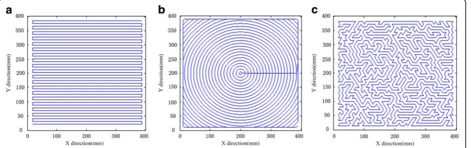
According to the CCOS principle, the path has marked influence on the MSF errors. Therefore, in this section the generation methods of various paths (i.e., raster path, circle path, random path) are stud-ied, and lay the foundation for the following experiments.
The flow of generating various paths mainly in-cludes the definition of variables, the definition of
variable initial value, the path selection, the calcula-tion of dwell point coordinates (xp, yp), the boundary
condition, and the output of dwell point coordinates. It should be pointed out that the main differences of three paths are the calculation formulas of dwell point coordinates, and the compendiary calculation formulas for raster path, circle path and random path are the Eqs. 3-5, respectively. Figure 2 shows the three paths that have been implemented.
xp¼xp−1þStep or xp¼xp−1−Step yp¼yp−1þPathSpacing
ð3Þ
Fig. 5aThe residual error map after the simulation andbthe contour in the X direction
xp¼r cos Angleð Þ yp ¼r sin Angleð Þ r¼r0:PathSpacing:rn PointNumber¼2pir=Step
Angle¼0:2pi=PointNumber:2pi 8 > > > > < > > > > :
ð4Þ
xp¼xp−1þdx cos Angle ið ð ÞÞ yp ¼yp−1þdx sin Angle ið ð ÞÞ dx¼ðPathSpacing=sqrtð Þ3 Þ 2 Angle¼pi=3:pi=3:2pi i¼randpermð6;1Þ 8 > > > > < > > > > :
ð5Þ
In Eqs. 3-5, (xp, yp) are the coordinates of the
dwell point, Step is the distance of adjacent dwell points on the path, Path spacing is the distance of adjacent path, r0 is the starting radius, rn is the
end-ing radius, and i is the sequence number of random direction. The random path has different travel di-rections, and the each travel direction selects by the random number i.
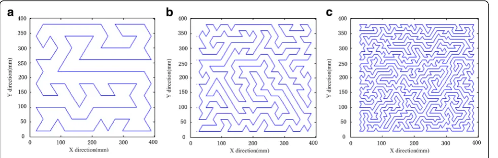
Figure 3 shows random paths with different path spacings. For workpieces of same size, the path spa-cing changes the density degree of path. The path spacing is small and the path is dense. From a dense random path, the path seems more random and may help improve the surface texture, which will be vali-dated in subsequent analysis. It should note that the path generated each time is totally different with an-other, as shown in Fig. 3. This reflects the random-ness of random path.
Surface topography simulation model
Figure 4 is a flowchart of surface topography simula-tion. In Fig. 4, firstly, enter the initial surface, the TIF, the path type and the path spacing. Secondly, the simulating surface topography is achieved by the iterative convolution calculation. At last, the PSD curve is calculated by the power spectral density
method, and the error distribution in a specified fre-quency band is calculated by the filter method.
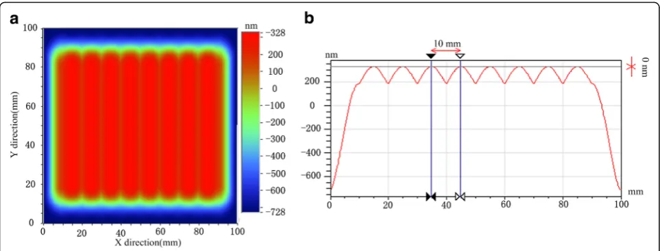
Surface topography simulation model is used to calculate the residual error with the Gaussian TIF and the raster path, and the MSF error is analyzed. In the simulation, the processing area is 100 mm × 100 mm, the TIF diameter is 20 mm, and the path spacing is 10 mm. Figure 5 shows the residual error map after the simulation and the contour in the X direction. Figure 6 illustrates the PSD curve of re-sidual error and the rere-sidual ripple distribution (50 mm × 50 mm).
It can be seen from Fig. 5 that there is a regular raster ripple (period 10 mm) consistent with the path spacing (10 mm) due to the effect of the con-volution effect in the raster path simulation process, and the PSD curve produces a significant peak (shown in the red circle position in Fig. 6(a)), whose frequency is 0.1 mm−1. This paper defines the fre-quency at a significant peak in the PSD curve as the characteristic frequency, whose amplitude is the PSD value of characteristic frequency (PSDc). Figure 6(b) shows the residual ripples in the middle region (50 mm × 50 mm) of the residual error. In this paper, the root-mean-square of residual ripple in the 50 mm × 50 mm region is defined as the RMS value of residual ripple (RMSr). In the following orthog-onal simulation and experiment, the PSDc and the RMSr are used to evaluate the effect of restraining the MSF errors.
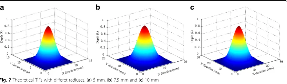
Fig. 7Theoretical TIFs with differet radiuses, (a) 5 mm, (b) 7.5 mm and (c) 10 mm
Table 1Level of each factor in orthogonal simulation experiment
Factor TIF diameter
mm
Path type Path spacing mm
Level 1 20 raster 4
2 15 circle 3
Conditions and results
Orthogonal simulation experiments
Three main factors, the TIF diameter, the path type and the path spacing, are considered in orthogonal simulation. The TIF is assumed to be the Gaussian type (shown in Fig. 7). The path types include raster path, circle path, and random path with path spacing of 2, 3 and 4 mm. In addition, the error of initial surface is 0, and its size is 100 mm × 100 mm. To ensure the comparability of results, the simulation results are normalized. The RMSr and the PSDc under unit removal depth are used as evaluative indexes, mean-while the RMSr and PSDc are calculated within the band filter for 0.5 mm-10 mm. The level of each factor is shown in Table 1. The simulation conditions and results are
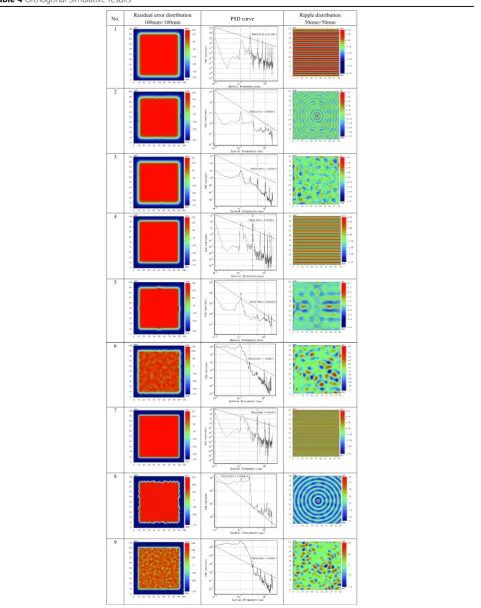
shown in Table 2. The surface simulation results under various combined parameters, including the residual error distribution (100 mm × 100 mm), PSD curve, and the ripple distribution (50 mm × 50 mm) are shown in Appendix 1.
In simulation experiment, the TIF is assumed to be Gaussian type, shown as follow,
R xð ;yÞ ¼A exp −x 2þy2
r 2 2
" #
ð6Þ
In Eq. 6, A is the adjustment factor of amplitude, and r is the radius of TIF, xϵ(−r, r), yϵ(−r, r). When A is assumed as 1 and r is assumed as 5 mm,
Fig. 8Actual TIFs with differet radiuses, (a) 4.5 mm, (b) 7.25 mm and (c) 9.5 mm
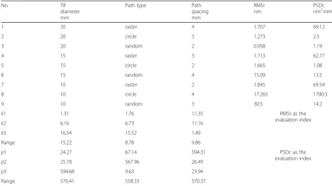
Table 2Simulative conditions and results
No. TIF
diameter mm
Path type Path
spacing mm
RMSr nm
PSDc nm2·mm
1 20 raster 4 1.707 69.12
2 20 circle 3 1.273 2.5
3 20 random 2 0.958 1.19
4 15 raster 3 1.713 62.77
5 15 circle 2 1.665 1.08
6 15 random 4 15.09 13.5
7 10 raster 2 1.845 69.54
8 10 circle 4 17.265 1700.3
9 10 random 3 30.5 14.2
k1 1.31 1.76 11.35 RMSr as the
evaluation index
k2 6.16 6.73 11.16
k3 16.54 15.52 1.49
Range 15.22 8.78 9.86
p1 24.27 67.14 594.31 PSDc as the
evaluation index
p2 25.78 567.96 26.49
p3 594.68 9.63 23.94
7.5 mm, 10 mm, the corresponding theoretical TIFs are shown in Fig. 7(a), (b), and (c), respectively.
Practical polishing experiments
In order to verify the influence of parameter com-bination on the MSF error further, the practical orthogonal experiments are carried out. The condi-tions in the practical experiments are consistent with the orthogonal simulation experiments and a self-developed bonnet polishing machine was adopted. When the bonnet radius R = 80 mm is used, the actual TIF with the two compressions, i.e., 0.65 and 0.35 mm, can be obtained, as shown in Fig. 8(a) and (b). And their actual radius is 4.5 and 7.25 mm re-spectively. When the bonnet radius R = 40 mm is used, the actual TIF with the compression 0.3 mm
can be obtained, as shown in Fig. 8(c), and its actual radius is 9.5 mm. The experiment conditions and re-sults are shown in Table 3. The practical polishing results under various combined parameters, includ-ing the residual error distribution (100 mm × 100 mm), PSD curve, and the ripple distribution (50 mm × 50 mm) are shown in Appendix 2.
Discussion
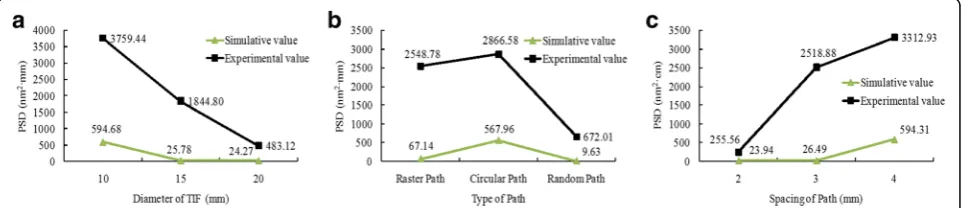
Influence of process parameter combination on PSDc According to Tables 2 and 3, the PSDc values in the simulation and practical experiments are drawn in Fig. 9.
Figure 9 shows that each factor has the same ten-dency to the evaluative index (PSDc) in simulation and experiment. However, it is necessary to point
Fig. 9Influence of various factors on PSDc, (a) TIF diameter, (b) path type and (c) path spacing
Table 3Experimental conditions and results
No. TIF
diameter mm
Path type Path
spacing mm
RMSr nm
PSDc nm2·mm
1 20 raster 4 7.838 1384
2 20 circle 3 3.285 53.43
3 20 random 2 3.23 4.68
4 15 raster 3 13.858 5570
5 15 circle 2 3.274 10.24
6 15 random 4 18.152 14.89
7 10 raster 2 7.199 913
8 10 circle 4 25.513 8311
9 10 random 3 25.718 1955
k1 4.78 9.63 17.17 RMSr as the
evaluation index
k2 11.76 10.69 14.29
k3 19.48 15.70 4.57
Range 14.69 5.01 12.60
p1 480.70 2622.33 3236.63 PSDc as the
evaluation index
p2 1865.04 2791.56 2526.14
p3 3726.33 658.19 309.31
out that the simulation results under each set of pa-rameters are smaller than the experimental results. The possible reason is that there is a difference be-tween the simulated and actual polishing process. The simulation is based on the TIF of Gaussian type and the linear removal model, while in the polishing process, the TIF has the shape distortion influenced by the instability of polishing conditions, i.e., polish-ing fluid, tool condition and polishpolish-ing environment. Actually, the TIF is time-varying in the practical pol-ishing process.
According to the orthogonal simulation and experimental results, the influence of process param-eters on the PSDc from three aspects are discussed in this section.
(1)Influencing degree of the parameters: in Tables2 and3, it shows that the ranges of PSDc values of TIF diameter in the simulation and practical experiments are maximal, and their value are 570.41 nm2·mm, 3245.63 nm2·mm, respectively. While the ranges of PSDc values of path type in the simulation and practical experiments are minimal, and their value are 558.33 and 2133.37 nm2·mm. According to the ranges of PSDc of parameters, it is shown that the
parameters in descending order of impact are as follows: TIF diameter, path spacing, and path type. (2)Optimal combined parameters: according to Fig.9,
the simulation and experimental results show that the combined parameters, i.e., 20 mm of TIF diameter, 2 mm of path spacing, and random path, can obtain the minimal PSDc, which is considered to be an optimal combination in the selected parameters. (3)Relationship between parameters and evaluative
index: it can be seen from Fig.9, the influences of parameters on the evaluative index (PSD value) is that, the larger the TIF diameter is, and the smaller
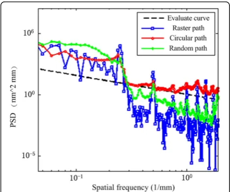
the path spacing is, the smaller the PSDc is, otherwise the path types in descending order of impact are as follows: random path, raster path, and circle path. Figure10shows the surface generation by different path types, i.e., raster path, circle path and random path. According to Fig.10, the PSD curves by three path types are calculated, shown in Fig.11.
Orthogonal analysis determines that the random path has the optimal ability to restrain the PSDc. The random path is an unicursal path with three random direction angles (i.e., 60°, 120°, and 180°). In the processing process, it will produce the ripples in three directions, i.e., 60°, 120°, and 180°. Although the random path also has a certain regularity, which is slighter than the raster and circle path, so the regular ripple will be suppressed, that is, the PSDc consistent with the path spacing is suppressed.
Fig. 11Comparison of PSD curves by three path types
Influence of process parameter combination on RMSr According to Tables 2 and 3, the RMSr values in the simulation and practical experiments are drawn in Fig. 12.
Figure 12 illustrates the comparisons between the mea-sured and the simulated results about the RMS of ripple under various conditions. It shows that the simulated ripple exhibits a good agreement with the practical measured rip-ple. However, the simulation results are smaller than the experimental results. The reason may be consistent with the previous analysis in “Influence of process parameter combination on PSDc” section, which is due to the deteri-oration of MSF error caused by the instability of processing conditions during the actual process. The dynamic factors will be investigated to improve the removal determinism in further study which is not within the scope for this paper.
According to the orthogonal simulation and experimental results, the influence of process parameters on the RMSr from three aspects are discussed in this section.
(1)Influencing degree of the parameters: in Tables 2 and3, it shows that the ranges of RMSr values of TIF diameter in the simulation and practical experiments are maximal, and their value are 15.22 and 14.69 nm, respectively. While
the ranges of RMSr values of path type in the simulation and practical experiments are minimal, and their value are 8.78 nm, 5.01 nm, respectively. According to the ranges of RMSr of parameters, we can see that the parameters in descending order of impact are as follows: TIF diameter, path spacing, and path type.
(2)Optimal combined parameters: according to Fig.12, the simulation and experimental results show that the combined parameters, i.e., 20 mm of TIF diameter, 2 mm of path spacing, and raster path, can obtain the minimal RMSr, which is considered to be an optimal combination in the selected parameters.
The optimized parameters obtained in this part are inconsistent with the“Influence of process parameter combination on PSDc”section, mainly due to the different evaluation indexes used in the two sections, which are PSDc and RMSr respectively. In the actual processing, in order to ensure that the two evaluation indexes can be qualified, the two sets of optimized parameters can be used alternately.
(3)Relationship between parameters and evaluative index: it can be seen from Fig.12, the influences of parameters on the RMSr is that, the larger the TIF diameter is, the smaller the path spacing is and the
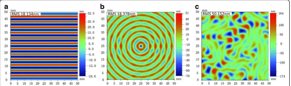
Fig. 13Contours of residual ripples with three paths, (a) raster path, (b) circle path and (c) random path
smaller the RMSr is, otherwise the path types in descending order of impact are as follows: raster path, circle path, and random path.
The influence of TIF diameter and path spacing on the ripples is similar to the previous research results [13]. The following analysis focuses on the influence of path type on the RMSr. Figure13shows the contours of residual ripples with three paths, i.e., raster path, circle path, random path, with keeping other process parameters consistent. Figure14is the curves of residual ripples with three paths. It can be seen from Fig.14that the ripple amplitude of raster path is minimal, and the ripple amplitude of circle path is slightly larger than that of raster path, and the ripple amplitude of random path is maximal. According to the characters of three paths, it shows that the ripple feature is related to the turn angle on the path. When the angle between the dwell points on the path is less than 180°, the extra removal exhibits on the corner. Theoretically, the turn angle on the raster path is 180 °, and the turn angle between the dwell points on
the circle path is related to the radius of circle. The smaller the radius is, the more extra removal is, so the residual ripple of circle path is slightly larger than the raster path, and is prone to produce“center error”at the center of circle path. Since the turn angle is generally large (more than 90°), the extra removal produced by the circle path is not significant. There are three angles, such as 60°, 120°, and 180° between the dwell points on the random path. Comparing the removal depth at the corner with different angles, the removal depth with corner angle 60° is the maximal, and the removal depth with corner angle 180° is the minimal, as shown in Fig.15. Since the RMSr is directly related to the amplitude of ripple, the raster path produces the minimum ripple, while the random path produces the maximum ripple.
Conclusions
A surface topography simulation model for the generation of MSF errors has been established. A model-based simula-tion system, which involves the theoretic TIF model, path planning methods and removal model etc., can forecast the surface topography with the various combined parameters, and export the CNC programs used in the practical polish-ing experiments. Orthogonal simulation experiments were designed for the following three parameters, i.e., TIF diam-eter, path type, and path spacing, and verified through the practical polishing experiments. The RMSr and the PSDc were used to evaluate the simulations and experiments. The two evaluative indexes are both improved with the in-crease of TIF diameter or the dein-crease of path spacing. The random path can reduce the PSDc, but worsen the RMSr, while the influences of raster path on the two evaluative in-dexes are opposite to those of random path. In addition, the parameters in descending order of impact on the MSF errors are as follows: TIF diameter, path spacing, and path type. Therefore, in order to control the MSF errors, the optimization of TIF diameter is the top-priority strategy.
Fig. 15Excess removal at corner of random path, (a) random path and (b) surface generation by random path
Appendix 1
Appendix 2
Abbreviations
BP:Bonnet Polishing; CCOS: Computer-controlled optical surfacing; IBF: Ion Beam Figuring; LLNL: Lawrence Livermore National Laboratory;
MRF: Magnetorheological Finishing; MSF: Mid-spatial-frequency; NIF: National Ignition Facility Project; PJM: Plasma Jet Machining; PSD: Power spectral density; PSDc: PSD value of characteristic frequency; RMS: Root-mean-square; RMSr: RMS value of residual ripple; TIF: Tool influence function
Acknowledgements Not applicable.
Funding
This work was financially supported by the Science Challenge Project (No. JCKY2016212A506-0502) and the Youth Talent Fund of Laser Fusion Research Center, CAEP. (No. RCFCZ1-2017-6).
Availability of data and materials Data will be shared after publication.
Authors’contributions
BZ and HH developed the surface topography simulation model; XC, WD and JW assisted conducting the experiments. All authors read and approved the final manuscript.
Ethics approval and consent to participate Not applicable.
Consent for publication Not applicable.
Competing interests
The authors have declared that no competing interests exist.
Publisher’s Note
Springer Nature remains neutral with regard to jurisdictional claims in published maps and institutional affiliations.
Received: 13 December 2017 Accepted: 8 February 2018
References
1. Spaeth, M.L., Manes, K.R., Widmayer, C.C., Williams, W., Whitman, P.A., Henesian, M.: The National Ignition Facility Wavefront Requirements and optical architecture. Proc. SPIE.5341, 25–42 (2004)
2. Yu, G., Li, H., Walker, D.D.: Removal of mid spatial-frequency features in mirror segments. J. Eur. Opt. Soc.6, 11044 (2011)
3. Glatzel, H., Ashworth, D., Bremer, M., Chin, R., Cummings, K., Girard, L., Goldstein, M., Gullikson, E., Hudyma, R., Kennon, J., Kestner, B., Marchetti, L., Naulleau, P., Soufli, R., Spiller, E.: Projection optics for extreme ultraviolet lithography (EUVL) micro-field exposure tools (METs) with a numerical aperture of 0.5. Proc of. SPIE.8679, 867917 (2013)
4. Shafrir, S.N., Lambropoulos, J.C., Jacobs, S.D.: A magnetorheological polishing-based approach for studying precision microground surfaces of tungsten carbides. Precis. Eng.31(2), 83–93 (2007)
5. Arnold, T., Pietag, F.: Ion beam figuring machine for ultra-precision silicon spheres correction. Precis. Eng.41, 119–125 (2015)
6. Arnold, T., Boehm, G., Paetzelt, H.: New freeform manufacturing chain based on atmospheric plasma jet machining. J. Eur. Opt. Soc.11, 16002 (2016) 7. Walker, D.D., Brooks, D., King, A., Freeman, R., Morton, R., McCavana, G., Kim,
S.: The‘precessions’tooling for polishing and figuring flat, spherical and aspheric surfaces. Opt. Express.11(8), 958–964 (2003)
8. Li, H.Y., Yu, G.Y., Walker, D.D., Evans, R.: Modelling and measurement of polishing tool influence. J. Eur. Opt. Soc.6, 11048 (2011)
9. Walker, D.D., Yu, G., Bibby, M., Dunn, C., Li, H., Wu, H.Y., Zheng, X., Zhang, P.: Robotic automation in computer controlled polishing. J. Eur. Opt. Soc.11, 16005 (2016) 10. Feit, M.D., Rubenchik, A.M.: Influence of subsurface cracks on laser induced
surface damage. Proc. SPIE.5273, 264–272 (2004)
11. Lawson, J.K., Wolfe, C.R., Manes, K.R., Trenholme, J.B., Aikens, D.M., English Jr., R.E.: Specification of optical components using the power spectral density function. Proc of. SPIE.2536, 38–50 (1995)
12. Pohl, M., Börret, R.: Simulation of mid-spatials from the grinding process. J. Eur. Opt. Soc.11, 16010 (2016)
13. Wang, C.J., Yang, W., Ye, S., Wang, Z.Z., Zhong, B., Guo, Y.B., Xu, Q.: Optimization of parameters for bonnet polishing based on the minimum residual error method. Opt. Eng.53(7), 075108 (2014)
14. Wang, C., Yang, W., Ye, S., Wang, Z.Z., Yang, P., Peng, Y., Guo, Y., Xu, Q.: Restraint of tool path ripple based on the optimization of tool step size for sub-aperture deterministic polishing. Int. J. Adv. Manuf. Technol.75, 1431–1438 (2014) 15. Wang, C.J., Wang, Z., Xu, Q.: Unicursal random maze tool path for
computer-controlled optical surfacing. Appl. Opt.54(34), 10128–10136 (2015) 16. Wang, T., Cheng, H.B., Yang, H., Wu, W.T., Tam, H.Y.: Controlling mid-spatial
frequency errors in magnetorheological jet polishing with a simple vertical model. Appl. Opt.54(21), 6433–6440 (2015)
17. Tam, H.Y., Cheng, H.B., Dong, Z.C.: Peano-like paths for subaperture polishing of optical aspherical surfaces. International journal of advanced manufacturing technology. Appl. Opt.52(15), 3624–3636 (2015) 18. Tam, H.Y., Cheng, H.B.: An investigation of the effects of the tool path on the
removal of material in polishing. J. Mater. Process. Technol.210, 807–818 (2010) 19. Khakpour, H., Birglen, L., Tahan, S.: Uniform scanning path generation for
abrasive waterjet polishing of free-form surfaces modeled by triangulated meshes. Int. J. Adv. Manuf. Technol.77, 1167–1176 (2015)
20. Dunn, C.R., Walker, D.D.: Pseudo-random tool paths for CNC sub-aperture polishing and other applications. Opt. Express.16(23), 18942–18949 (2008) 21. Hu, H., Dai, Y.F., Peng, X.Q.: Restraint of tool path ripple based on surface
error distribution and process parameters in deterministic finishing. Opt. Express.18(22), 22973–22981 (2010)