ESTIMATING RETURNS TO SCALE USING NON-RADIAL DEA MODELS
M. ALLAHYAR1∗, M. ROSTAMY-MALKHALIFEH2, M. MIRBOLOUKI1,§
Abstract. The concept of returns to scale (RTS) is defined as the ratio of the propor-tionate changes in outputs over the proporpropor-tionate changes in inputs. By considering the following two facts the current paper develops some non-radial data envelopment analy-sis (DEA) models to address a new concept of RTS termed the component RTS :a) The proportionate changes in input will not necessarily cause the proportionate changes in outputs; b) If it is desired for decision maker (DM) to find out about the rate of increase in a specific component of output vector after exerting changes in inputs, the radial-based models will not be able to make this wish come true. In other words, the main objective of this work is to seek the disproportionate changes, coming in to existence in any individual components of output vector, through exerting changes on inputs of under evaluation unit. The suggested models are used in a case study that is focused on RTS estimation of some bank branches.Keywords: Data Envelopment Analysis (DEA), Efficiency, Radial and non-radial model, Returns To Scale (RTS).
AMS Subject Classification: 90BXX, 90B15, 90CXX, 90C15.
1. Introduction
Data envelopment analysis (DEA) is a non-parametric technique based on mathematical programming for the performance assessment of a set of decision making units (DMUs). Charnes et al. [6] and Banker et al. [2] presented CCR (Charnse, Cooper, Rhodes) and BCC (Banker, Charnse, Cooper) models respectively as the basic DEA models. The con-cept of returns to scale (RTS) is one of the subjects that have allocated a wide contribution of DEA literature to itself. DEA classifies DMUs to three groups according to their RTS status: Constant RTS (CRS), increasing RTS (IRS) and decreasing RTS (DRS). So far, there have been several attempts to estimate this notion based on formal DEA models (see, e.g. [3], [5], [17], [20], [16], [15]). There are a few review papers which detail differ-ent basic methods in the RTS literature such as [4]. Actually, the efficiency analysis and estimating RTS are among the most important management actions for the performance assessment and assessing the optimal size of units. In other words, determining the RTS behavior can provide useful information by which decision maker (DM) can improve the productivity of efficient units by resizing the scale of their operations.
1∗
Young Researchers and Elite Club, Yadegar-e-Imam Khomeini (RAH) Shahre Rey Branch, Islamic Azad University, Tehran, Iran.
e-mail: allahyar [email protected]; ORCID: https://orcid.org/0000-0002-3291-0442. e-mail: [email protected]; ORCID: https://orcid.org/ 0000-0003-1054-8208.
2
Department of Mathematics, Science and Research Branch, Islamic Azad University, Tehran, Iran. e-mail: mohsen [email protected]; ORCID: https://orcid.org/0000-0001-6105-7674.
§ Manuscript received: September 18, 2016; accepted: June 1, 2017.
TWMS Journal of Applied and Engineering Mathematics, Vol.8, No.1a cI¸sık University, Department of Mathematics, 2018; all rights reserved.
Reviewing the customary methods, we could find out that the RTS estimation by theme holds only in the current position of the under study unit. For example, these methods may identify CRS for an extreme unit lying on the efficient frontier, whereas DRS and IRS prevail at a close right and left neighborhood of this unit respectively. With respect to this point, the right and left RTS notions were first addressed by Golany and Yu [10] and they proposed an approach based on solving two LP models. In fact, they addressed the RTS status in a close neighborhood of the under evaluation unit instead of its current position. However, this method fails when at least one of the models is infeasible. It is worth mentioning that [12] as well as [1] have provided a remedy to overcome this short-coming. There are few papers which discuss the right and left RTS. See, e. g., [19]. In actual fact, RTS are defined based on the magnitude of the ratio of the proportionate changes in outputs over the proportionate changes in inputs which are sometimes referred to as scale elasticity in economics. Examples of methods for the calculation of scale elas-ticity can be found in DEA literature ([8], [11], [9], [14], [21]). It should not be forgotten that; first, the proportionate changes in input will not necessarily cause the proportionate changes in outputs; second, if, for instance, it is desired for DM to find out about the rate of increase in specific component of output vector after exerting changes in inputs, the radial models will not be able to make this wish come true. In current paper we consider RTS related to each component of output vector separately through some suggested non-oriented models. There are some attempts in DEA literature which determine RTS in the non-radial models. See, for example, [4] and [18]. In fact, their methods are based on the optimal solutions obtained from Range-Adjusted Model (RAM) ([7]). The advantage of our method over the mentioned methods is that it is based on the optimal value of the objective function of suggested non-radial models. Therefore, even in the presence of multiple optimal solutions, the new method is able to measure RTS. It must be noted that [13] developed an approach to investigate the elasticity of a subset of outputs with respect to marginal changes of a subset of inputs.
Banking industry plays a vital role in the nation’s economy. To validate our method we present a real-world application to the banking industry, which is one of the most signifi-cant application areas of DEA. The process of this practice involves the estimation of RTS related to the efficient units and research on how these could be improved.
The rest of this paper is structured as follows: In section 2, first we survey the preliminary definition of the right and left RTS and then introduce two LP models. Section 3 gives details of the main results of the paper. Section 4 will use a real data to illustrate the suggested method. Finally, Section 5 contains some conclusions.
2. The right and left returns to scale
Suppose we have a set of n DMUs. Each DM Uj (j=1,...,n) consumes the input vector
Xj = (x1j, ..., xmj) to produce output vectorYj = (y1j, ..., ysj). The production possibility set (PPS) under variable returns to scale is expressed as follows:
Tv =
(
(X, Y)|Pn
j=1
λjXj ≤X, n
P
j=1
λjYj ≥Y , λj ≥0, j = 1, ..., n
)
.
Consider an efficient unit identified by BCC model, say, DM Uo whose coordinate is (Xo, Yo).
ρ+
o = lim θ→1+
γ(θ)−1
θ−1 ,ρ
−
o = lim θ→1−
γ(θ)−1
θ−1 (1)
Where the parameterθassumes a positive arbitrary value andγ(θ) corresponding DMUo is
γ(θ) = max{γ|(θX0, γY0)∈TV}. (2)
Assumption 1. There areθ∈[0,1) andγ ≥0 such that (θX0, γY0)∈TV.
Evidently, formula (1) is the right and left derivatives of the function γ(θ) atθ= 1. Ac-cording to concavity of the efficient frontier, the proportional increase in input of DMUo is possible in Tv, i.e. ρ+o is always defined.
Lemma 2.1. if γ(1) = 1 and Assumption 1 holds then ρ−o is defined.
Proof. See lemma 2.3 in [11].
Definition 2.1. The RTS to the right of DM Uo is IRS (DRS, CRS) if ρ+o >1(ρ+o <1,
ρ+o = 1) and the RTS to the left ofDM Uo is IRS (DRS, CRS) ifρ−o >1(ρ−o <1, ρ−o = 1). Definition 2.2. The RTS of the DM Uo is IRS (DRS) if ρ+o > 1, ρ−o > 1 (ρ+o < 1,
ρ−o <1). In other cases CRS prevails for DM Uo.
In order to estimate RTS to the right and left neighborhood ofDM Uo, we present two following models respectively:
β∗=M axβ
s.t.
n
P
j=1
λjxj ≤(1 +δ)xo
n
P
j=1
λjyj ≥βyo
n
P
j=1 λj = 1
λj ≥0j = 1, . . . , n
(1)
and
α∗ =M axα
s.t.
n
P
j=1
µjxj ≤(1−η)xo
n
P
j=1
µjyj ≥αyo
n
P
j=1 µj = 1
µj ≥0j= 1, . . . , n
(2)
It should be noted that Model (1) is one of the two models presented in [1]. This model is feasible for each DMU, whereas Model (2) that is similar to the model presented by [10], is infeasible for some special DMUs. To overcome this shortcoming, we can apply the algorithm suggested in [12]. In fact, through this approach, the interval (0, η∗] is de-fined as the assurance interval for feasibility of Model (2), if this model is feasible for each
η∈(0, η∗]. The following model is used for obtaining this interval:
η∗= M ax η
s.t.
n
P
j=1
µjxj ≤(1−η)xo
n
P
j=1
µjyj ≥αyo
n
P
j=1 µj = 1
µj ≥0j= 1, . . . , n
(3)
Lemma 2.2. η∗= 0 if and only if Model (3) is feasible.
Proof. See lemma 1 in [12].
Theorem 2.1. The following conditions identify the state of the right RTS ofDM Uo via
Model (1): 1(i) If (1 +δ)> β∗ >1 ⇒ DRS 1(ii) If(1 +δ)< β∗ ⇒ IRS
1(iii) If(1 +δ) = β∗ ⇒ CRS
Proof. We prove only case 1(i), and the other cases can be proved similarly. Suppose (β∗, λ∗1, ..., λ∗n) be the optimal solution of Model (1) and condition (1 +δ) > β∗ > 1 is satisfied. So, according relation (1) and since the value ofδ is selected sufficiently small, we have:
ρ+0 = lim
(1+δ)→1+ β∗−1 (1+δ)−1 <1
Then, regarding Definition 2.1., RTS to the right ofDM Uo is IRS.
Theorem 2.2. The following conditions identify the state of the left RTS of DM Uo via
Model (2):
2(i) Ifα∗ <(1−η) ⇒ IRS 2(ii) If(1−η)< α∗ <1 ⇒ DRS 2(iii) Ifα∗ = (1−η) ⇒ CRS
2(iv) If the model is infeasible (η∗ = 0) ⇒ IRS
Proof. We prove only case 2(i), and the other cases can be proved similarly. Suppose (α∗, µ∗1, ..., µn∗) be the optimal solution of Model (2) and condition α∗ <(1−η) prevails. So, according relation (1) and since the value ofη is selected sufficiently small, we have:
ρ−0 = lim
(1−η)→1−
α∗−1 (1−η)−1 >1
3. Component Returns To Scale (CRTS)
It is evident that the results obtained from Theorems 2.1. and 2.2. are based on the maximum proportional changes occurred in outputs after solving Models (1) and (2) re-spectively. Considering this feature, if DM were interested in being informed about the state of RTS related to the especial components of output vector, then none of these mod-els would be able to respond this request. Focusing on this point, we introduce a new concept of RTS in the next section. In this section we investigate RTS in more details, introducing a new concept named the component return to scale (CRTS) introducing two non- radial DEA model.
Adapting Definition 2.1., consider the following relations:
ρ+
ro = lim θ→1+
γr(θ)−1
θ−1 ,ρ
−
ro= lim θ→1−
γr(θ)−1
θ−1 (3)
Where γr(θ) corresponding the rth component of output vector of DM Uo (i.e. yro ) is
γr(θ) = max{γr|(θx1o, ..., θxmo, γ1y1o, ..., γryro, ..., γsyso)∈Tv,(γ1, ..., γr, ..., γs)≥1} (4) Where 1 is a vector with all components equal to one.
Definition 3.1. The right RTS of DM Uo related to yro is IRS (DRS, CRS) if ρ+ro >1, (ρ+ro <1, ρ+ro = 1). And the left RTS ofDM Uorelated to yro is IRS (DRS, CRS) ifρ−ro >1 (ρ−ro <1, ρ−ro = 1).
Definition 3.2. RTS of DM Uo is IRS (DRS) if ρ+ro > 1, ρ−ro > 1 (ρ+ro < 1, ρ−ro < 1).
Otherwise RTS ofDM Uo is CRS.
In continue, to estimate RTS classification for DM Uo related to yto(t=1,..., s) we sug-gest two following DEA models:
βtt∗ =M axβtt s.t.
n
P
j=1
λjxij ≤
1 + ˆδ
xio i= 1, . . . , m
n
P
j=1
λjyrj ≥βtryro r= 1, . . . , s
n
P
j=1 λj = 1
βrt ≥1r = 1, . . . .s λj ≥0j = 1, . . . , n
(4)
and
αtt∗ =M axαtt s.t.
n
P
j=1
µjxij ≤(1−bη)xio i= 1, . . . , m
n
P
j=1
µjyrj ≥αtryro r= 1, . . . , s
n
P
j=1 µj = 1
αtr≤1r = 1, . . . , s µj ≥0 j= 1, . . . , n
(5)
Theorem 3.1. The following conditions identify the state of the right CRTS of DM Uo
related to yto via Model (4):
3(i) If(1 + ˆδ)> βtt∗ ⇒ DRS 3(ii ) If(1 + ˆδ)< βtt∗ ⇒ IRS 3(iii) If(1 + ˆδ) =βtt∗ ⇒ CRS
Proof. We prove only case 3(i), and the other cases can be proved similarly. Suppose (λ∗1, ..., λ∗n, β1t∗, ..., βtt∗, ..., βst∗) be the optimal solution of Model (4) and condition (1 + ˆδ)> βtt∗ is satisfied. So, according relation (3) and since the value of ˆδ is selected sufficiently small, we have:
ρ+ro = lim
(1+ˆδ)→1+ βtt∗−1
(1+ˆδ)−1 <1
Then, regarding Definition 3.1., CRTS to the right ofDM Uo related toyto is DRS.
Theorem 3.2. The following conditions identify the state of the left CRTS of DM Uo
related to yto via Model (5):
4(i) If(1−ηˆ)> αtt∗ ⇒ IRS 4(ii) If(1−ηˆ)< αtt∗ ⇒ DRS 4(iii) If(1−ηˆ) =αtt∗ ⇒ CRS
4(iv) If the model is infeasible ⇒ IRS
Proof. We prove only case 4(i), and the other cases can be proved similarly. Suppose (µ∗1, ..., µ∗n, αt1∗, ..., αtt∗, ..., αts∗) be the optimal solution of Model (5) and condition (1−ηˆ)> αtt∗ is satisfied. So, according relation (3) and the value of ˆη is selected sufficiently small, we have:
ρ−ro = lim
(1−ηb)→1
−
αt∗ t −1
(1−bη)−1
>1
Then, regarding Definition 3.1., CRTS to the right ofDM Uo related toyto is DRS.
4. Applications to bank branch data
To illustrate the applicability and efficacy of the proposed method, we here consider 20 bank branches with two inputs and three outputs listed in Table 1. In our application, we estimate RTS corresponding to each efficient branch by which the manager could reform the system to obtain the optimal size. Table 2 shows data.
The reasons why we have chosen these inputs and outputs are listed below:
1. Since equities of each branch mean the sum of the value of the bank’s assets, the amount of equities are considered as an input.
2. Since the human resources assigned to the branches in order to obtain more output and since this costs money, the personnel are considered as input.
3. Bank credit is the aggregation of funds provided to individuals. A high credit score indicates a stronger credit profile. So the amount of the credit can be considered as an output.
4. Because the amount of customers’ deposits is the result of the branch activities, deposits are considered as output.
benefit is an income and considered as an output.
It should be noted that in this research we consider the indexes which have the most important impacts on the performance of the branches.
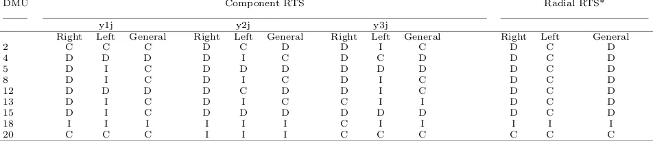
The state of the right and left RTS in every component of output vector (Component RTS) and the radial RTS via the suggested models are reported in Tables 3. Where C, I and D indicate constant, increasing and decreasing RTS respectively. The general RTS is also determined through the following definition.
Definition 4.1. The general RTS of a DMU is DRS (IRS) if both RTS to the left and RTS to the right are DRS (IRS). Otherwise, its general RTS is CRS.
Implications and suggestions:
The decision maker of a banking unit is willing to be informed of the RTS behavior to determine whether the unit can improve its productivity by resizing the scale of its oper-ations. If results show the presence of DRS for large branches, manager could potentially improve outcomes by limiting the activities and size of these units. When there is IRS, the branch’s average cost of production is decreasing, i.e. more than increase in the amount of input output increases. When there is CRS it means that economic profit is zero in the long run.
Here there are some important suggestions based on the obtained results.
For instance, Table 3 shows the presence of constant right component RTS for the first output and decreasing right component RTS for the second and third output of DMU2. It means increasing the related inputs of this branch yields growth in deposit and benefit, but not as big as growth in credit. On the other hand, by considering three different weight vectors whose components show the desired weight of manager related to each output, decreasing prevail for this branch. So, it is recommended that the manager apply an ap-propriate strategy considering the emphasis he laid on each component of output vector. For example, in our application, if credit has preference over the deposit and profit and this branch is able to increase its size by bank policies, the increase in the size of branch 2 can be appropriate.
Indeed, returns to scale have a positive effect on productivity growth. In case the existence any of the RTS status, the following strategies have been suggested:
DRS: Limiting the size and activity to reduce the average cost IRS: Increasing the size and activity as much as possible
CRS: making change cautiously (after careful deliberation)
In sum, if the decision maker of a banking system is willing to extend the size of the bank, then he should either create a new branch or increase the size and activity of the branches that have increasing RTS.
5. Conclusion
But the difference is that our suggested method is based on non-radial models and assigns a coefficient to each output component separately.
References
[1] Allahyar M., Rostamy-Malkhalifeh M. (2015). “An improved approach for estimating returns to scale in DEA”.Bull Malays Math Sci Soc. 37(4), 1185-1194.
[2] Banker R.D., Charnes A., Cooper W. W. (1984). “Some models for estimating technical and scale efficiencies in date envelopment analysis”.Manage Sci. 30, 1078-1092.
[3] Banker R.D. (1984). “ Estimating most productive scale size using data envelopment analysis”. Eur J Oper Res. 17, 35-44.
[4] Banker R.D., Cooper W.W., Thrall R.M., Seiford L.M., Zhu J. (2004). “Returns to scale in different DEA models”.Eur J Oper Res. 154, 345-362.
[5] Banker R.D., Thrall R.M. (1992). “Estimation of returns to scale using date envelopment analysis”.
Eur J Oper Res. 62, 74-84.
[6] Charnes A., Cooper W.W., Rhodes E. (1978). “Measuring the efficiency of decision making units”.
Eur J Oper Res. 2, 429-444.
[7] Cooper W.W., Park K.S., Pastor J.T. (2000). “RAM: A range adjusted measure of efficiency”.J Prod Anal. 11, 5-42.
[8] Forsund F.R. (1996). “On the calculation of scale elasticities in DEA models”.J Prod Anal. 7, 283-302 [9] Forsund F.R., Hjalmarsson L., Krivonozhko V.E., Utkin O.B. (2007). “Calculation of scale elasticities
in DEA models: Direct and indirect approaches”.J Prod Anal. 28, 45-56.
[10] Golany B., Yu G. (1997). “Estimating returns to scale in DEA”.Eur J Oper Res. 103, 28-37. [11] Hadjicostas P., Soteriou A.C. (2006). “One-sided elasticities and technical efficiency in multi-output
production: A theoretical framework”.Eur J Oper Res. 198, 425-449.
[12] Jahanshahloo G.R., Soleimani-damaneh M., Rostamy-Malkhalifeh M. (2005). “An enhanced procedure for estimating returns-to-scale in DEA”.Appl Math Comput. 171, 1226-1238.
[13] Podinovski V.V., Fosund F.R. (2010). “Differential characteristics of efficient frontiers in data envel-opment analysis”.Oper Res. 58, 1743-1754.
[14] Podinovski V.V., Forsund F.R., Krivonozhko V.E. (2009). “A simple derivation of scale elasticity in data envelopment analysis”.Eur J Oper Res. 197, 149-153.
[15] Soleimani-Damaneh M. (2012). “On a basic definition of returns to scale”.Oper Res Lett. 40, 144-147. [16] Soleimani-damaneh M., Jahanshahloo G.R., Reshadi M. (2006). “On the estimation of returns to scale
in FDH models”.Eur J Oper Res. 174(2), 1055-1059.
[17] Tone K. (2001). “On returns to scale under weights restrictions in data envelopment analysis”.J Prod Anal. 16, 31-47.
[18] Krivonozhko V.E., Forsund F.R., Lychev A.V. (2014). “Measurement of returns to scale using non-radial DEA models”.Eur J Oper Res. 232, 664-670.
[19] Zarepisheh M., Soleimani-damaneh M. (2009). “A dual simplex-based method for determination of the right and left returns to scale in DEA”.Eur J Oper Res. 194, 585-591.
[20] Zarepisheh M., Soleimani-damaneh M., Pourkarimi L. (2006). “Determination of returns to scale by CCR formulation without chasing down alternative optimal solutions”.Appl Math Lett. 19(9), 964-967. [21] Zelenyuk V. (2013). “A scale elasticity measure for directional distance function and its dual: Theory
and DEA estimation”.Eur J Oper Res. 228, 592-600.
Tables
Table 1. Inputs and outputs
Input1 amount of equity
Input2 personnel (number off employee)
Output1 amount of the credit
Table 2. Data for 20 bank branches
DMU Equity(x1) Staff(x2) Credit(y1) Deposit(y2) Profit(y3)
1 255 41 184 482 118
2 382 47 539 700 455
3 691 119 487 638 370
4 425 101 784 863 687
5 931 105 1015 319 650
6 537 106 437 742 499
7 785 72 752 681 193
8 256 13 323 611 154
9 362 102 652 481 156
10 186 87 648 535 89
11 358 86 234 805 133
12 776 93 488 958 693
13 88 47 761 653 97
14 892 52 472 470 320
15 556 40 848 658 325
16 199 113 364 147 57
17 158 61 503 549 127
18 78 128 184 225 91
19 268 95 673 432 219
20 322 32 544 368 309
Table 3. The classification of component RTS and radial RTS for efficient DMUs
DMU Component RTS Radial RTS*
y1j y2j y3j
Right Left General Right Left General Right Left General Right Left General
2 C C C D C D D I C D C D
4 D D D D I C D C D D C D
5 D I C D D D D D D D C D
8 D I C D I C D I C D C D
12 D D D D C D D I C D C D
13 D I C D I C C I I D C D
15 D I C D D D D D D D C D
18 I I I I I I C I I I I I
20 C C C I I I C C C C C C
* The right and left radial RTS is estimated through models (3) and (4) respectively.
Maryam Allahyar holds a Ph.D. in operations research. She is a lecturer at the Department of Mathematics, Yadegar-e-Imam Khomeini (RAH) Shahre Rey Branch, Islamic Azad University, Tehran, Iran. Her research interests include Operations Research and Data Envelopment Analysis.
Mohsen Rostamy-Malkhalifeh is an associate professor at the Department of Mathematics, Science and Reserach Branch, Islamic Azad University, Tehran, Iran. His main research interests are related to Operations Research and Data Envelopment Analysis.